Psychometrics Archives

What is the two parameter IRT model (2PL)?

Nathan Thompson, PhDNovember 28, 2018

Item response theory is the predominant psychometric paradigm for mid or large scale assessment. As noted in my introductory blog post, it is actually a family of models. In this post, we discuss the two parameter IRT model (IRT 2PL).

Consider the following 3PL equation (simplified from Hambleton & Swaminathan, 1985, Eq. 3.3). The IRT 2PL simply removes the c and (1-c) elements, so that probability is only a function of a and b.

This equation is predicting the probability of a certain response based on the examinee trait/ability level, the item discrimination parameter a, and the item difficulty/location parameter b. If the examinee’s trait level is higher than the item location, the person has more than a 50% chance of responding in the keyed direction.

This phrase “in the keyed direction” is one you might often hear with the IRT 2PL. This is because it is not often used with education/knowledge/ability assessments where items usually have a correct answer and guessing is often possible. The IRT 2PL is used more often in attitudinal or other psychological assessments where guessing is irrelevant and there is no correct answer. For example, consider an Extroversion scale, where examinees are responding Yes/No to statements like “I love to go to parties” or “I prefer to read books in my free time.” There is not much to guess here, and the sense of “correct” is not relevant.

However, it is quite clear that the first statement is keyed in the direction of extroversion while the second statement is the reverse. In fact, you would get the 1 point of response for saying No to that statement rather than Yes. This is often called reverse-scored.

There are other aspects that go into whether you should use the 2PL model, but this is one of the most important. In addition, you should also examine model fit indices and take sample size into account.

How do I implement the two parameter IRT model?

Like other IRT models, the 2PL requires specialized software. Not all statistical packages will do it. And while you can easily calculate classical statistics in Excel, there is no way to do IRT (well, unless you want to write your own VBA programs to do so). As mentioned in this article on the three parameter model, there are a lot of IRT software programs available, but not all meet the required standards.

You should evaluate cost and functionality. If you are a fan of R, there are packages to estimate IRT there. However, I recommend our Xcalibre program for both newbies and professionals. For newbies, it is much easier to use, which means you spend more time learning the concepts of IRT and not fighting command code that might be 30 years old. For professionals, Xcalibre saves you from having to create reports by copy and paste which is incredibly expensive.

November 28, 2018/by Nathan Thompson, PhD

What is the three parameter IRT model (3PL)?

Nathan Thompson, PhDNovember 28, 2018

Item response theory (IRT) is an extremely powerful psychometric paradigm that addresses many of the inadequacies of classical test theory (CTT). If you are new to the topic, there is a broad intro here, where you will learn that IRT is actually a family of mathematical models rather than one specific one. Today, I’m talking about the 3PL.

One of the most commonly used models is called the three parameter IRT model (3PM), or the three parameter logistic model (3PL or 3PLM) because it is almost always expressed in a logistic form. The equation for this is below (Hambleton & Swaminathan, 1985, Eq. 3.3).

Like all IRT models, it is seeking to predict the probability of a certain response based on examinee ability/trait level and some parameters which describe the performance of the item. With the 3PL, those parameters are a (discrimination), b (difficulty or location), and c (pseudo-guessing). For more on these, check out the descriptions in my general IRT article.

The remaining point then is what we mean by the probability of a certain response. The 3PL is a dichotomous model which means that it is predicting a binary outcome such as correct/incorrect or agree/disagree.

When should I use the three parameter IRT model?

The applicability of the 3PL to a certain assessment depends on the relevance of the components just discussed. First, the response to the items must be binary. This eliminates Likert-type items (“Rate on a scale of 1 to 5”), partial credit items (scoring an essay as 0 to 5 points), and performance assessments where scoring might include a range of points, deductions, or timing (number of words typed per minute).

Next, you should evaluate the applicability of the use of all three parameters. Most notably, are the items in your assessment susceptible to guessing? Because the thing that differentiates the 3PL from its sisters the 1PL and 2PL is that it attempts to model for guessing. This, of course, is highly relevant for multiple-choice items on knowledge or ability assessments, so the 3PL is often a great fit for those.

Even in this case, though, there are a number of practitioners and researchers that still prefer to use the 1PL or 2PL models. There are some deeper methodological issues driving this choice. The 2PL is sometimes chosen because it works well with an estimation method called Joint Maximum Likelihood.

The 1PL, also known as the Rasch model (yes, I know the Rasch people will say they are not the same, I am grouping them together for simplicity in comparison), is often selected because adherents to the model believe in certain advantages such as it providing “objective measurement.” Also, the Rasch model works far better for smaller samples (see this technical report by Guyer & Thompson and this one by Yoes). Regardless, you should probably evaluate model fit when selecting models.

I am from a camp that is pragmatic in choice rather than dogmatic. While training on the 3PL in graduate school, I have no qualms against using the 2PL or 1PL/Rasch if the test type and sample size warrant it or if fit statistics indicate they are sufficient.

How do I implement the three parameter IRT model?

If you want to implement the three parameter IRT model, you need specialized software. General statistical software such as SPSS does not always produce IRT analysis, though some do. Even in the realm of IRT-specific software, not all produce the 3PL. And, of course, the software can vary greatly in terms of quality. Here are three important ways it can vary:

Accuracy of results: check out this research study which shows that some programs are inaccurate
User-friendliness: some programs require you to write extensive code, and some have a purely graphical interface
Output usability and interpretability: some programs just give simple ASCII text, others provide extensive Word or HTML reports with many beautiful tables and graphs.

For more on this topic, head over to my post on how to implement IRT in general.

Want to get started immediately? Download a free copy of our IRT software Xcalibre.

November 28, 2018/by Nathan Thompson, PhD

What is classical item facility?

Nathan Thompson, PhDOctober 28, 2018

Classical test theory is a century-old paradigm for psychometrics – using quantitative and scientific processes to develop and analyze assessments to improve their quality. (Nobody likes unfair tests!) The most basic and frequently used item statistic from classical test theory is the P-value. It is usually called item difficulty but is sometimes called item facility, which can lead to possible confusion.

The P-Value Statistic

The classical P-value is the proportion of examinees that respond correctly to a question, or respond in the “keyed direction” for items where the notion of correct is not relevant (imagine a personality assessment where all questions are Yes/No statements such as “I like to go to parties” … Yes is the keyed direction for an Extraversion scale). Note that this is NOT the same as the p-value that is used in hypothesis testing from general statistical methods. This P-value is almost universally agreed upon in terms of calculation. But some people call it item difficulty and others call it item facility. Why?

It has to do with the clarity interpretation. It usually makes sense to think of difficulty as an important aspect of the item. The P-value presents this, but in a reverse manner. We usually expect higher values to indicate more of something, right? But a P-value of 1.00 is high, and it means that there is not much difficulty; everyone gets the item correct, so it is actually no difficulty whatsoever. A P-value of 0.25 is low, but it means that there is a lot of difficulty; only 25% of examinees are getting it correct, so it has quite a lot of difficulty.

So where does “item facility” come in?

See how the meaning is reversed? It’s for this reason that some psychometricians prefer to call it item facility or item easiness. We still use the P-value, but 1.00 means high facility/easiness, and 0.25 means low facility/easiness. The direction of the semantics fits much better.

Nevertheless, this is a minority of psychometricians. There’s too much momentum to change an entire field at this point! It’s similar to the 3 dichotomous IRT parameters (a, b, c); some of you might have noticed that they are actually in the wrong order because the 1-parameter model does not use the parameter, it uses the b.

At the end of the day, it doesn’t really matter, but it’s another good example of how we all just got used to doing something and it’s now too far down the road to change it. Tradition is a funny thing.

October 28, 2018/by Nathan Thompson, PhD

Setting a cutscore to item response theory

Nathan Thompson, PhDAugust 2, 2018

Need to set a cutscore on a test with item response theory? There are ways to do so directly, such as the Bookmark method. But do you have an existing cutscore on the number-correct scale? Cutscores set with classical test theory, such as the Angoff, Nedelsky, or Ebel methods, are easy to implement when the test is scored classically. But if your test is scored with the item response theory (IRT) paradigm, you need to convert your cutscores onto the theta scale. The easiest way to do that is to reverse-calculate the test response function (TRF) from IRT. This post will discuss that.

The Test Response Function

The TRF (sometimes called a test characteristic curve) is an important method of characterizing test performance in the IRT paradigm. The TRF predicts a classical score from an IRT score, as you see below. Like the item response function and test information function (item response and test information function ), it uses the theta scale as the X-axis. The Y-axis can be either the number-correct metric or proportion-correct metric.

In this example, you can see that a theta of -0.4 translates to an estimated number-correct score of approximately 7. Note that the number-correct metric only makes sense for linear or LOFT exams, where every examinee receives the same number of items. In the case of CAT exams, only the proportion correct metric makes sense.

Classical cutscore to IRT

So how does this help us with the conversion of a classical cutscore? Well, we hereby have a way of translating any number-correct score or proportion-correct score. So any classical cutscore can be reverse-calculated to a theta value. If your Angoff study (or Beuk) recommends a cutscore of 7 out of 10 points, you can convert that to a theta cutscore of -0.4 as above. If the recommended cutscore was 8, the theta cutscore would be approximately 0.7.

Because IRT works in a way that it scores examinees on the same scale with any set of items, as long as those items have been part of a linking/equating study. Therefore, a single study on a set of items can be equated to any other linear test form, LOFT pool, or CAT pool. This makes it possible to apply the classically-focused Angoff method to IRT-focused programs.

August 2, 2018/by Nathan Thompson, PhD

Linear on the fly testing

Nathan Thompson, PhDAugust 2, 2018

Linear on the fly testing (LOFT) is an approach to assessment delivery that increases test security by limiting item exposure. It tries to balance the advantages of linear testing (e.g., everyone sees the same number of items, which feels fairer) with the advantages of algorithmic exams (e.g., creating a unique test for everyone).

In general, there are two families of test delivery. Static approaches deliver the same test form or forms to everyone; this is the ubiquitous and traditional “linear” method of testing. Algorithmic approaches deliver the test to each examinee based on a computer algorithm; this includes LOFT, computerized adaptive testing (CAT), and multistage testing (MST).

What is linear on-the-fly testing?

The purpose of linear on the fly testing is to give every examinee a linear form that is uniquely created for them – but each one is created to be psychometrically equivalent to all others to ensure fairness. For example, we might have a pool of 200 items, and every person only gets 100, but that 100 is balanced for each person. This can be done by ensuring content and/or statistical equivalency, as well ancillary metadata such as item types or cognitive level.

Content Equivalence

This portion is relatively straightforward. If your test blueprint calls for 20 items in each of 5 domains, for a total of 100 items, then each form administered to examinees should follow this blueprint. Sometimes the content blueprint might go 2 or even 3 levels deep.

Statistical Equivalence

There are, of course, two predominant psychometric paradigms: classical test theory (CTT) and item response theory (IRT). With CTT, forms can easily be built to have an equivalent P value, and therefore expected mean score. If point-biserial statistics are available for each item, you can also design the algorithm to design forms that have the same standard deviation and reliability.

With item response theory, the typical approach is to design forms to have the same test information function, or inversely, conditional standard error of measurement function. To learn more about how these are implemented, read this blog post about IRT or download our Classical Form Assembly Tool.

Implementing LOFT

LOFT is typically implemented by publishing a pool of items with an algorithm to select subsets that meet the requirements. Therefore, you need a psychometrically sophisticated testing engine that stores the necessary statistics and item metadata, lets you define a pool of items, specify the relevant options such as target statistics and blueprints, and deliver the test in a secure manner. Very few testing platforms can implement a quality LOFT assessment. ASC’s platform does; click here to request a demo.

Why all this?

It certainly is not easy to build a strong item bank, design LOFT pools, and develop a complex algorithm that meets the content and statistical balancing needs. So why would an organization use linear on the fly testing?

Well, it is much more secure than having a few linear forms. Since everyone receives a unique form, it is impossible for words to get out about what the first questions on the test are. And of course, we could simply perform a random selection of 100 items from a pool of 200, but that would be potentially unfair. Using LOFT will ensure the test remains fair and defensible.

August 2, 2018/by Nathan Thompson, PhD

What is the Hofstee method for setting cutscores?

Nathan Thompson, PhDMay 23, 2018

Have you heard about standard setting approaches such as the Hofstee method, or perhaps the Angoff, Ebel, Nedelsky, or Bookmark methods? There are certainly various ways to set a defensible cutscore or a professional credentialing or pre-employment test. Today, we are going to discuss the Hofstee method.

Why Standard Setting?

Certification organizations that care about the quality of their examinations need to follow best practices and international standards for test development, such as the Standards laid out by the National Commission for Certifying Agencies (NCCA). One component of that is standard setting, also known as cutscore studies. One of the most common and respected approaches for that is the modified-Angoff methodology.

However, the Angoff approach has one flaw: the subject matter experts (SMEs) tend to expect too much out of minimally competent candidates, and sometimes set a cutscore so high that even they themselves would not pass the exam. There are several reasons this can occur. For example, raters might think “I would expect anyone that worked for me to know how to do this” and not consider the fact that people who work for them might have 10 years of experience while test candidates could be fresh out of training/school and have the topic only touched on for 5 minutes. SMEs often forget what it was like to be a much younger and inexperienced version of themselves.

For this reason, several compromise methods have been suggested to compare the Angoff-recommended cutscore with a “reality check” of actual score performance on the exam, allowing the SMEs to make a more informed decision when setting the official cutscore of the exam. I like to use the Beuk method and the Hofstee method.

The Hofstee Method

One method of adjusting the cutscore based on raters’ impressions of the difficulty of the test and possible pass rates is the Hofstee method (Mills & Melican, 1987; Cizek, 2006; Burr et al., 2016). This method requires the raters to estimate four values:

The minimum acceptable failure rate
The maximum acceptable failure rate
The minimum cutscore, even if all examinees failed
The maximum cutscore, even if all examinees passed

The first two values are failure rates, and are therefore between 0% and 100%, with 100% indicating a test that is too difficult for anyone to pass. The latter two values are on the raw score scale, and therefore range between 0 and the number of items in the test, again with a higher value indicating a more difficult cutscore to achieve.

These values are paired, and the line that passes through the two points estimated. The intersection of this line with the failure rate function, is the recommendation of the adjusted cutscore.

How can I use the Hofstee Method?

Unlike the Beuk, the Hofstee method does not utilize the Angoff ratings, so it represents a completely independent reality check. In fact, it is sometimes used as a standalone cutscore setting method itself, but because it does not involve rating of every single item, I recommend it be used in concert with the Angoff and Beuk approaches.

May 23, 2018/by Nathan Thompson, PhD

What is the Spearman-Brown formula?

Nathan Thompson, PhDApril 14, 2018

The Spearman-Brown formula, also known as the Spearman-Brown Prophecy Formula or Correction, is a method used in evaluating test reliability. It is based on the idea that split-half reliability has better assumptions than coefficient alpha but only estimates reliability for a half-length test, so you need to implement a correction that steps it up to a true estimate for a full-length test.

Looking for software to help you analyze reliability? Download a free copy of Iteman.

Coefficient Alpha vs. Split Half

The most commonly used index of test score reliability is coefficient alpha. However, it’s not the only index on internal consistency. Another common approach is split-half reliability, where you split the test into two halves (first/last, even/odd, or random split) and then correlate scores on each. The reasoning is that if both halves of the test measure the same construct at a similar level of precision and difficulty, then scores on one half should correlate highly with scores on the other half. More information on split-half is found here.

However, split-half reliability provides an inconvenient situation: we are effectively gauging the reliability of half a test. It is a well-known fact that reliability is increased by more items (observations); we can all agree that a 100-item test is more reliable than a 10 item test comprised of similar quality items. So the split half correlation is blatantly underestimating the reliability of the full-length test.

The Spearman-Brown Formula

To adjust for this, psychometricians use the Spearman-Brown prophecy formula. It takes the split half correlation as input and converts it to an estimate of the equivalent level of reliability for the full-length test. While this might sound complex, the actual formula is quite simple.

As you can see, the formula takes the split half reliability (r_half) as input and produces the full-length estimation (r_full) . This can then be interpreted alongside the ubiquitously used coefficient alpha.

While the calculation is quite simple, you still shouldn’t have to do it yourself. Any decent software for classical item analysis will produce it for you. As an example, here is the output of the Reliability Analysis table from our Iteman software for automated reporting and assessment intelligence with CTT. This lists the various split-half estimates alongside the coefficient alpha (and its associated SEM) for the total score as well as the domains, so you can evaluate if there are domains that are producing unusually unreliable scores.

Note: There is an ongoing argument amongst psychometricians whether domain scores are even worthwhile since the assumed unidimensionality of most tests means that the domain scores are less reliable estimates of the total score, but that’s a whole ‘another blog post!

Score	N Items	Alpha	SEM	Split-Half (Random)	Split-Half (First-Last)	Split-Half (Odd-Even)	S-B Random	S-B First-Last	S-B Odd-Even
All items	50	0.805	3.058	0.660	0.537	0.668	0.795	0.699	0.801
1	10	0.522	1.269	0.338	0.376	0.370	0.506	0.547	0.540
2	18	0.602	1.860	0.418	0.309	0.448	0.590	0.472	0.619
3	12	0.605	1.496	0.449	0.417	0.383	0.620	0.588	0.553
4	10	0.485	1.375	0.300	0.329	0.297	0.461	0.495	0.457

You can see that, as mentioned earlier, there are 3 ways to do the split in the first place, and Iteman reports all three. It then reports the Spearman-Brown formula for each. These generally align with the results of the alpha estimates, which overall provide a cohesive picture about the structure of the exam and its reliability of scores. As you might expect, domains with more items are slightly more reliable, but not super reliable since they are all less than 20 items.

So, what does this mean in the big scheme of things? Well, in many cases the Spearman-Brown estimates might not differ from the alpha estimates, but it’s still good to know that they do. In the case of high-stakes tests, you want to go through every effort you can to ensure that the scores are highly reliable and precise.

Tell me more!

If you’d like to learn more, here is an article on the topic. Or, contact solutions@assess.com to discuss consulting projects with our Ph.D. psychometricians.

April 14, 2018/by Nathan Thompson, PhD

What artificial intelligence and machine learning tell us about item banks?

Nathan Thompson, PhDMarch 29, 2018

Artificial intelligence (AI) and machine learning (ML) have become buzzwords over the past few years. As I already wrote about, they are actually old news in the field of psychometrics. Factor analysis is a classical example of ML, and item response theory also qualifies as ML. Computerized adaptive testing is actually an application of AI to psychometrics that dates back to the 1970s.

One thing that is very different about the world of AI/ML today is the massive power available in free platforms like R, Python, and TensorFlow. I’ve been thinking a lot over the past few years about how these tools can impact the world of assessment. A straightforward application is too automated essay scoring; a common way to approach that problem is through natural language processing with the “bag of words” model and utilize the document-term matrix (DTM) as predictors in a model for essay score as a criterion variable. Surprisingly simple. This got me to wondering where else we could apply that sort of modeling. Obviously, student response data on selected-response items provides a ton of data, but the research questions are less clear. So, I turned to the topic that I think has the next largest set of data and text: item banks.

Step 1: Text Mining

The first step was to explore tools for text mining in R. I found this well-written and clear tutorial on the text2vec package and used that as my springboard. Within minutes I was able to get a document term matrix, and in a few more minutes was able to prune it. This DTM alone can provide useful info to an organization on their item bank, but I wanted to delve further. Can the DTM predict item quality?

Step 2: Fit Models

To do this, I utilized both the caret and glmnet packages to fit models. I love the caret package, but if you search the literature you’ll find it has a problem with sparse matrices, which is exactly what the DTM is. One blog post I found said that anyone with a sparse matrix is pretty much stuck using glmnet.

I tried a few models on a small item bank of 500 items from a friend of mine, and my adjusted R squared for the prediction of IRT parameters (as an index of item quality) was 0.53 – meaning that I could account for more than half the variance of item quality just by knowing some of the common words in each item’s stem. I wasn’t even using the answer texts n-grams, or additional information like Author and content domain.

Want to learn more about your item banks?

I’d love to swim even deeper on this issue. If you have a large item bank and would like to work with me to analyze it so you can provide better feedback and direction to your item writers and test developers, drop me a message at solutions@assess.com! This could directly impact the efficiency of your organization and the quality of your assessments.

March 29, 2018/by Nathan Thompson, PhD

7 Technology Hacks to deliver assessments more securely

Nathan Thompson, PhDMarch 27, 2018

So, yeah, the use of “hacks” in the title is definitely on the ironic and gratuitous side, but there is still a point to be made: are you making full use of current technology to keep your tests secure? Gone are the days when you are limited to linear test forms on paper in physical locations. Here are some quick points on how modern assessment technology can deliver assessments more securely, effectively, and efficiently than traditional methods:

1. AI delivery like CAT and LOFT

Psychometrics was one of the first areas to apply modern data science and machine learning (see this blog post for a story about a MOOC course). But did you know it was also one of the first areas to apply artificial intelligence (AI)? Early forms of computerized adaptive testing (CAT) were suggested in the 1960s and had become widely available in the 1980s. CAT delivers a unique test to each examinee by using complex algorithms to personalize the test. This makes it much more secure, and can also reduce test length by 50-90%.

2. Psychometric forensics

Modern psychometrics has suggested many methods for finding cheaters and other invalid test-taking behavior. These can range from very simple rules like flagging someone for having a top 5% score in a bottom 5% time, to extremely complex collusion indices. These approaches are designed explicitly to keep your test more secure.

3. Tech enhanced items

Tech enhanced items (TEIs) are test questions that leverage technology to be more complex than is possible on paper tests. Classic examples include drag and drop or hotspot items. These items are harder to memorize and therefore contribute to security.

4. IP address limits

Suppose you want to make sure that your test is only delivered in certain school buildings, campuses, or other geographic locations. You can build a test delivery platform that limits your tests to a range of IP addresses, which implements this geographic restriction.

5. Lockdown browser

A lockdown browser is a special software that locks a computer screen onto a test in progress, so for example a student cannot open Google in another tab and simply search for answers. Advanced versions can also scan the computer for software that is considered a threat, like a screen capture software.

6. Identity verification

Tests can be built to require unique login procedures, such as requiring a proctor to enter their employee ID and the test-taker to enter their student ID. Examinees can also be required to show photo ID, and of course, there are new biometric methods being developed.

7. Remote proctoring

The days are gone when you need to hop in the car and drive 3 hours to sit in a windowless room at a community college to take a test. Nowadays, proctors can watch you and your desktop via webcam. This is arguably as secure as in-person proctoring, and certainly more convenient and cost-effective.

So, how can I implement these to deliver assessments more securely?

Some of these approaches are provided by vendors specifically dedicated to that space, such as ProctorExam for remote proctoring. However, if you use ASC’s FastTest platform, all of these methods are available for you right out of the box. Want to see for yourself? Sign up for a free account!

March 27, 2018/by Nathan Thompson, PhD

Monte carlo simulation in adaptive testing

Nathan Thompson, PhDFebruary 24, 2018

Simulation studies are an essential step in the development of a computerized adaptive test (CAT) that is defensible and meets the needs of your organization or other stakeholders. There are three types of simulations: monte carlo, real data (post hoc), and hybrid.

Monte Carlo simulation is the most general-purpose approach, and the one most often used early in the process of developing a CAT. This is because it requires no actual data, either on test items or examinees – although real data is welcome if available – which makes it extremely useful in evaluating whether CAT is even feasible for your organization before any money is invested in moving forward.

Let’s begin with an overview of how Monte Carlo simulation works before we return to that point.

How a Monte Carlo Simulation works: An Overview

First of all, what do we mean by CAT simulation? Well, a CAT is a test that is administered to students via an algorithm. We can use that same algorithm on imaginary examinees, or real examinees from the past, and simulate how well a CAT performs on them.

Best of all, we can change the specifications of the algorithm to see how it impacts the examinees and the CAT performance.

Each simulation approach requires three things:

Item parameters from item response theory, though new CAT methods such as diagnostic models are now being developed
Examinee scores (theta) from item response theory
A way to determine how an examinee responds to an item if the CAT algorithm says it should be delivered to the examinee.

The monte Carlo simulation approach is defined by how it addresses the third requirement: it generates a response using some sort of mathematical model, while the other two simulation approaches look up actual responses for past examinees (real-data approach) or a mix of the two (hybrid).

The Monte Carlo simulation approach only uses the response generation process. The item parameters can either be from a bank of actual items or generated.

Likewise, the examinee thetas can be from a database of past data, or generated.

How does the response generation process work?

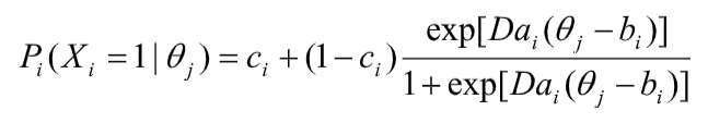
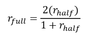
Well, it differs based on the model that is used as the basis for the CAT algorithm. Here, let’s assume that we are using the three-parameter logistic model. Start by supposing we have a fake examinee with a true theta of 0.0. The CAT algorithm looks in the bank and says that we need to administer item #17 as the first item, which has the following item parameters: a=1.0, b=0.0, and c=0.20.

Well, we can simply plug those numbers into the equation for the three-parameter model and obtain the probability that this person would correctly answer this item.

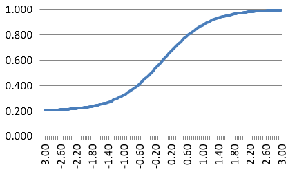
The probability, in this case, is 0.6. The next step is to generate a random number from the set of all real numbers between 0.0 and 1.0. If that number is less than the probability of correct response, the examinee “gets” the item correct. If greater, the examinee gets the item incorrect. Either way, the examinee is scored and the CAT algorithm proceeds.

For every item that comes up to be used, we utilize this same process. Of course, the true theta does not change, but the item parameters are different for each item. Each time, we generate a new random number and compare it to the probability to determine a response of correct or incorrect.

The CAT algorithm proceeds as if a real examinee is on the other side of the computer screen, actually responding to questions, and stops whenever the termination criterion is satisfied. However, the same process can be used to “deliver” linear exams to examinees; instead of the CAT algorithm selecting the next item, we just process sequentially through the test.

A road to research

For a single examinee, this process is not much more than a curiosity. Where it becomes useful is at a large scale aggregate level. Imagine the process above as part of a much larger loop. First, we establish a pool of 200 items pulled from items used in the past by your program. Next, we generate a set of 1,000 examinees by pulling numbers from a random distribution.

Finally, we loop through each examinee and administer a CAT by using the CAT algorithm and generating responses with the Monte Carlo simulation process. We then have extensive data on how the CAT algorithm performed, which can be used to evaluate the algorithm and the item bank. The two most important are the length of the CAT and its accuracy, which are a trade-off in most cases.

So how is this useful for evaluating the feasibility of CAT?

Well, you can evaluate the performance of the CAT algorithm by setting up an experiment to compare different conditions. Suppose you don’t have past items and are not even sure how many items you need? Well, you can create several different fake item banks and administer a CAT to the same set of fake examinees.

Or you might know the item bank to be used, but need to establish that a CAT will outperform the linear tests you currently use. There is a wide range of research questions you can ask, and since all the data is being generated, you can design a study to answer many of them. In fact, one of the greatest problems you might face is that you can get carried away and start creating too many conditions!

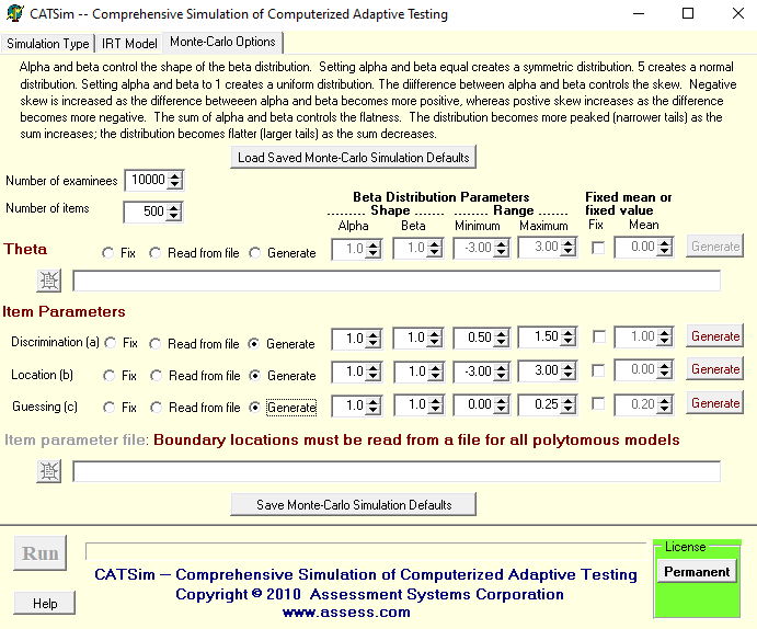
How do I actually do a Monte Carlo simulation study?

Fortunately, there is software to do all the work for you. The best option is CATSim, which provides all the options you need in a straightforward user interface (beware, this makes it even easier to get carried away). The advantage of CATSim is that it collates the results for you and presents most of the summary statistics you need without you having to calculate them. For example, it calculates the average test length (number of items used by a variable-length CAT), and the correlation of CAT thetas with true thetas. Other software exists which is useful in generating data sets using Monte Carlo simulation (see SimulCAT), but they do not include this important feature.

February 24, 2018/by Nathan Thompson, PhD