Posts on psychometrics: The Science of Assessment

response similarity index

Harpp, Hogan, and Jennings (1996) revised their Response Similarity Index somewhat from Harpp and Hogan (1993). This produced a new equation for a statistic to detect collusion and other forms of exam cheating: response similarity index.

Explanation of Response Similarity Index

EEIC denote the number of exact errors in common or identically wrong,

D is the number of items with a different response.

Note that D is calculated across all items, not just incorrect responses, so it is possible (and likely) that D>EEIC.  Therefore, the authors suggest utilizing a flag cutoff of 1.0 (Harpp, Hogan, & Jennings, 1996):

Analyses of well over 100 examinations during the past six years have shown that when this number is ~1.0 or higher, there is a powerful indication of cheating.  In virtually all cases to date where the exam has ~30 or more questions, has a class average <80% and where the minimum number of EEIC is 6, this parameter has been nearly 100% accurate in finding highly suspicious pairs.

However, Nelson (2006) has evaluated this index in comparison to Wesolowsky’s (2000) index and strongly recommends against using the HHJ.  It is notable that neither makes any attempt to evaluate probabilities or standardize.  Cizek (1999) notes that both Harpp-Hogan methods do not even receive attention in the psychometric literature.

This approach has very limited ability to detect cheating when the source has a high ability level. While individual classroom instructors might find the EEIC/D straightforward and useful, there are much better indices for use in large-scale, high-stakes examinations.

Harpp Hogan

Harpp and Hogan (1993) suggested a response similarity index defined as   

response similarity index by Harpp and Hogan (1993)


Response Similarity Index Explanation

EEIC denote the number of exact errors in common or identically wrong,

EIC is the number of errors in common.

This is calculated for all pairs of examinees that the researcher wishes to compare. 

One advantage of this approach is that it extremely simple to interpret: if examinee A and B each get 10 items wrong, 5 of which are in common, and gave the same answer on 4 of those 5, then the index is simply 4/5 = 0.80.  A value of 1.0 would therefore be perfect “cheating” – on all items that both examinees answered incorrectly, they happened to select the same distractor.

The authors suggest utilizing a flag cutoff of with the following reasoning (Harpp & Hogan, 1993, p. 307):

The choice of 0.75 is derived empirically because pairs with less than this fraction were not found to sit adjacent to one another while pairs with greater than this ratio almost always were seated adjacently.

The cutoff can differ from dataset to dataset, so SIFT allows you to specify the cutoff you wish to use for flagging pairs of examinees.  However, because this cutoff is completely arbitrary, a very high value (e.g., 0.95) is recommended by as this index can easily lead to many flaggings, especially if the test is short.  False positives are likely, and this index should be used with great caution.  Wesolowsky (unpublished PowerPoint presentation) called this method “better but not good.”

This index evaluates error similarity analysis (ESA), namely estimating the probability that a given pair of examinees would have the same exact errors in common (EEIC), given the total number of errors they have in common (EIC) and the aggregated probability P of selecting the same distractor.  Bellezza and Bellezza utilize the notation of k=EEIC and N=EIC, and calculate the probability

Bellezza and Bellezza calculate the probability

Note that this is summed from k to N; the example in the original article is that a pair of examinees had N=20 and k=18, so the equation above is calculated three times (k=18, 19, 20) to estimate the probability of having 18 or more EEIC out of 20 EIC.  For readers of the Cizek (1999) book, note that N and k are presented correctly in the equation but their definitions in the text are transposed.

The calculation of P is left to the researcher to some extent.  Published resources on the topic note that if examinees always selected randomly amongst distractors, the probability of an examinee selecting a given distractor is 1/d, where d is the number of incorrect answers, usually one less than the total number of possible responses.  Two examinees randomly selecting the same distractor would be (1/d)(1/d).  Summing across d distractors by multiplying by d, the calculation of P would be

error similarity analysis

That is, for a four-option multiple choice item, d=3 and P=0.3333.  For a five-option item, d=4 and P=0.25.

However, examinees most certainly do not select randomly amongst distractors. Suppose a four-option multiple-choice item was answered correctly by 50% (0.50) of the sample.  The first distractor might be chosen by 0.30 of the sample, the second by 0.15, and the third by 0.05.  SIFT calculates these probabilities and uses the observed values to provide a more realistic estimate of P

SIFT therefore calculates this error similarity analysis index using the observed probabilities and also the random-selection assumption method, labeling them as B&B Obs and B&B Ran, respectively.  The indices are calculated all possible pairs of examinees or all pairs in the same location, depending on the option selected in SIFT. 

How to interpret this index?  It is estimating a probability, so a smaller number means that the event can be expected to be very rare under the assumption of no collusion (that is, independent test taking).  So a very small number is flagged as possible collusion.  SIFT defaults to 0.001.  As mentioned earlier, implementation of a Bonferroni correction might be prudent.

The software program Scrutiny! also calculates this ESA index.  However, it utilizes a normal approximation rather than exact calculations, and details are not given regarding the calculation of P, so its results will not agree exactly with SIFT.

Cizek (1999) notes:

          “Scrutiny! uses an approach to identifying copying called “error similarity analysis” or ESA—a method which, unfortunately, has not received strong recommendation in the professional literature. One review (Frary, 1993) concluded that the ESA method: 1) fails to utilize information from correct response similarity; 2) fails to consider total test performance of examinees; and 3) does not take into account the attractiveness of wrong options selected in common. Bay (1994) and Chason (1997) found that ESA was the least effective index for detecting copying of the three methods they compared.”

Want to implement this statistic? Download the SIFT software for free.

frary g2

Estimated reading time: 3 minutes

The Frary, Tideman, and Watts (1977) g2 index is a collusion (cheating) detection index, which is a standardization that evaluates a number of common responses between two examinees in the typical standardized format: observed common responses minus the expectation of common responses, divided by the expected standard deviation of common responses.  It compares all pairs of examinees twice: evaluating examinee copying off b and vice versa.

Frary, Tideman, and Watts (1977) g2 Index

The g2 collusion index starts by finding the probability, for each item, that the Copier would choose (based on their ability) the answer that the Source actually chose.  The sum of these probabilities than the expected number of equivalent responses.  We can then compare this to the actual observed number of equivalent responses and standardize that difference with the standard deviation.  A very positive value could be possibly indicative of copying.


g2 collusion index

Where

Cab = Observed number of common responses (e.g., both examinees selected answer D)

k = number of items i

Uia = Random variable for examinee a’s response to item i

Xia = Observed response of examinee b to item i.

Frary et al. estimated P using classical test theory, and the definitions are provided in the original paper, while a slightly more clear definitions are provided in Khalid, Mehmood, and Rehman (2011).

The g2 approach produces two half-matrices, which SIFT presents as a single matrix separated by a blank diagonal.  That is, the lower half of the matrix evaluates whether examinee a copied off b, and the upper half whether b copied off a.  More specifically, the row number is the copier and the column number is the source.  So Row1/Column2 evaluates whether 1 copied off 2, while Row2/Column1 evaluates whether 2 copied off 1.

For g2 and Wollack’s (1997) ω, the flagging procedure counts all values in the matrix greater than the critical value, so it is possible – likely actually – that each pair will be flagged twice.  So the numbers in those flag total columns will be greater than those in the unidirectional indices.

How to interpret?  This collusion index is standardized onto a z-metric, and therefore can easily be converted to the probability you wish to use.  A standardized value of 3.09 is default for g2, ω, and Zjk because this translates to a probability of 0.001.  A value beyond 3.09 then represents an event that is expected to be very rare under the assumption of no collusion.

Want to implement this statistic? Download the SIFT software for free.

Wollack Omega

Wollack (1997) adapted the standardized collusion index of Frary, Tidemann, and Watts (1977) g2 to item response theory (IRT) and produced the Wollack Omega (ω) index.  It is clear that the graphics in the original article by Frary et al. (1977) were crude classical approximations of an item response function, so Wollack replaced the probability calculations from the classical approximations with those from IRT. 

The probabilities could be calculated with any IRT model.  Wollack suggested Bock’s Nominal Response Model since it is appropriate for multiple-choice data, but that model is rarely used in practice and very few IRT software packages support it.  SIFT instead supports the use of dichotomous models: 1-parameter, 2-parameter, 3-parameter, and Rasch.

Because of using IRT, implementation of ω requires additional input.  You must include the IRT item parameters in the control tab, as well as examinee theta values in the examinee tab.  If any of that input is missing, the omega output will not be produced.

The ω index is defined as

standardized collusion index of Frary, Tidemann, and Watts (1977) g2

Where P is the probability of an examinee with θa selecting the response, that examinee b selected, and cab is the RIC.  That is, the probability that the copier with θa would select the responses that the source did when summed, this can be interpreted as the expected RIC

Note: This uses all responses, not just errors.

How to interpret?  The value will be higher when the copier had more responses in common with the source than we’d expect from a person of that (probably lower) ability.  This index is standardized onto a z-metric, and therefore can easily be converted to the probability you wish to use. 

A standardized value of 3.09 is the default for g2, ω, and Zjk because this translates to a probability of 0.001.  A value beyond 3.09, then, represents an event that is expected to be very rare under the assumption of no collusion.

Interested in applying the Wollack Omega index to your data? Download the SIFT software for free.

wesolosky

Wesolowsky’s (2000) index is a collusion detection index, designed to look for exam cheating by finding similar response vectors amongst examinees. It is in the same family as g2 and Wollack’s ω.  Like those, it creates a standardized statistic by evaluating the difference between observed and expected common responses and dividing by a standard error.  It is more similar to the g2 index in that it is based on classical test theory rather than item response theory.  This has the advantage of being conceptually simpler as well as more feasible for small samples (it is well-known that IRT requires minimum sample sizes of 100 to 1000 depending on the model).  However, this of course means that it lacks the conceptual, theoretical, and mathematical appropriateness of IRT, which is the dominant psychometric paradigm for large-scale tests for good reason.

Wesolowsky defined his collusion detection index as

Wesolowsky collusion detection index

where

Here, the expected number of common responses  is equal to the joint probability of each examinee (j and k) getting item i correct, plus both getting it incorrect with the same distractor t selected.  This is calculated as a single probability for each item then summed across items.  The probability for each item is then of course multiplied by one minus itself to create a binomial variance.

The major difference between this and g2 is that g2 estimated the probability using a piecewise linear function that grossly approximated an item response function from IRT.  Wesolowsky utilized a curvilinear function he called “iso-contours” which is better in that it is curvilinear, but it is still not on par with the item response function in terms of conceptual appropriateness.  The iso-contours are described by a parameter Wesolowsky referred to as a (completely unrelated to the IRT discrimination parameter), which must be estimated by bisection approximation.

How to interpret?  This index is standardized onto a z-metric, and therefore can easily be converted to the probability you wish to use.  A standardized value of 3.09 is default for g2, ω, and Zjk because this translates to a probability of 0.001.  A value beyond 3.09 then represents an event that is expected to be very rare under the assumption of no collusion.

Want to calculate this index? Download the free program SIFT.

response-time-effort

Wise and Kong (2005) defined an index to flag examinees not putting forth minimal effort, based on their response time.  It is called the response time effort (RTE) index. Let K be the number of items in the test. The RTE for each examinee j is

response time effort

where TCji is 1 if the response time on item i exceeds some minimum cutpoint, and 0 if it does not. 

How do I interpret Response Time Effort?

This therefore evaluates the proportion of items for which the examinee spent less time than the specified cutpoint, and therefore ranges from 0 to 1. You, as the researcher, needs to decide what that cutpoint is: 10 second, 30 seconds… what makes sense for your exam?  It is then interpreted as an index of examinee engagement.  If you think that each item should take at least 20 seconds to answer (perhaps an average of 45 seconds), and Examinee X took less than 20 seconds on half the items, then clearly they were flying through and not giving the effort that they should.  Examinees could be flagged like this for removal from calibration data.  You could even use this in real time, and put a message on the screen “Hey, stop slacking, and answer the questions!”

How do I implement RTE?

Want to calculate Response Time Effort on your data? Download the free software SIFT.  SIFT provides comprehensive psychometric forensics, flagging examinees with potential issues such as poor motivation, stealing content, or copying amongst examinees.

Holland K

The Holland K index and variants are probability-based indices for psychometric forensics, like the Bellezza & Bellezza indices, but make use of conditional information in their calculations. All three estimate the probability of observing  wij  or more identical incorrect responses (that is, EEIC, exact errors in common) between a pair of examinees in a directional fashion. This is defined as

Holland K.

Here, Ws is the number of items answered incorrectly by the source, Wcs is the EEIC, and Pr is the probability of the source and copier having the same incorrect response to an item.  So, if the source had 20 items incorrect and the suspected copier had the same answer for 18 of them, we are calculating the probability of having 18 EEIC (the right side), then multiplying it by the number of ways there can be 18 EEICs in a set of 20 items (the middle).  Finally, we do the same for 19 and 20 EEIC and sum up our three values.  In this example, that would likely be summing three very small values because Pr is being taken to large powers and it is a probability such as 0.4.  Such a situation would be very unlikely, so we’d expect a K index value of 0.000012.

If there were no cheating, the copier might have only 3 EEIC with the source, and we’d be summing from 3 up to 20, with the earlier values being relatively large. We’d likely then end up with a value of 0.5 or more.

The key number here is the Pr. The three variants of the K index differ in how it is calculated. Each of them starts by creating a raw frequency distribution of EEIC for a given source to determine an expected probability at a given “score group” r defined by the number of incorrect responses. 

key number

Here, MW refers to the mean number of EEIC for the score group and Ws is still the number of incorrect responses for the source.

The K index (Holland, 1996) uses this raw value. The K1 index applies linear regression to smooth the distribution, and the K2 index applies a quadratic regression to smooth it (Sotaridona & Meijer, 2002); because the regression-predicted value is then used, the notation becomes M-hat.  Since these three then only differ by the amount of smoothing used in an intermediate calculation, the results will be extremely close to one another. This frequency distribution could be calculated based on only examinees in the same location, however, SIFT uses all examinees in the data set, as this would create a more conceptually appealing null distribution.

S1 and S2 apply the same framework of the raw frequency distribution of EEIC, but apply it to a different probability calculation instead of using a Poisson model:

S1 index.

S2 is often glossed over in publications as being similar, but it is much more complex.  It contains the Poisson model but calculates the probability of the observed EEIC plus a weighted expectation of observed correct responses in common. This makes much more logical sense because many of the responses that a copier would copy from a smarter student will, in fact, be correct. 

All the other K variants ignore this since it is so much harder to disentangle this from an examinee knowing the correct answer. Sotaridona and Meijer (2003), as well as Sotaridona’s original dissertation, provide treatment on how this number is estimated and then integrated into the Poisson calculations.

psychometrician in code

A psychometrician is someone who studies the process of assessment, namely how to develop and validate exams, regardless of the type of assessment (certification, employment, university admissions, K-12, etc.).  They are familiar with the scientific literature devoted to the development of fair, high-quality assessments, and they use this knowledge to improve assessments.  They implement aspects of engineering, data science, and machine learning to ensure that tests provide accurate information about people, so we can make decisions.

Request a meeting with a psychometric consultant


What is a Psychometrician?

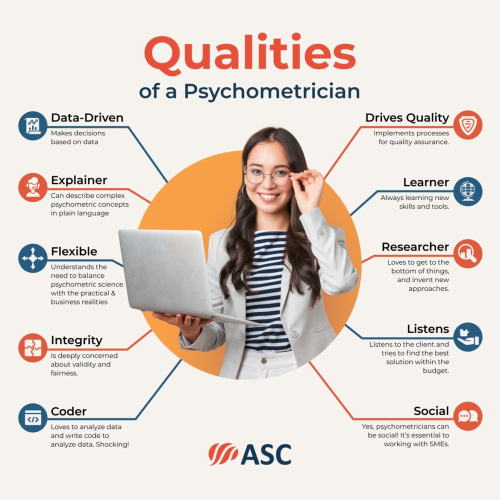
A psychometrician is like a lead engineer, applying best practices to produce a complex product that is reliable and serves the purpose of the test, such as predicting job performance.  This involves planning, management of a team of specialists, ensuring quality control, and other leadership.  However, psychometricians are often the type that like to get their hands dirty by writing code and analyzing data themselves.

In some parts of the world, the term psychometrician refers to someone who administers tests, typically in a counseling setting, and does not actually know anything about the development or validation of tests.  That usage is incorrect; such a person is a psychometrist, as you can see at the website for the here.  Even major sites like ZipRecruiter don’t do the basic fact-checking to get this straight.


Psychometrician Qualities

What does a psychometrician do?

There are many steps that go into developing a high quality, defensible assessment.  These differ by the purpose of the test.  When working on professional certifications or employment tests, a job analysis is typically necessary and is frequently done by a psychometrician.  Yet job analysis totally irrelevant for K-12 formative assessments; the test is based on a curriculum, so a psychometrician’s time is spent elsewhere.

Some topics include:

This is a highly quantitative profession.  Psychometricians spend most of their time working with datasets, using specially designed software or writing code in languages like R and Python.

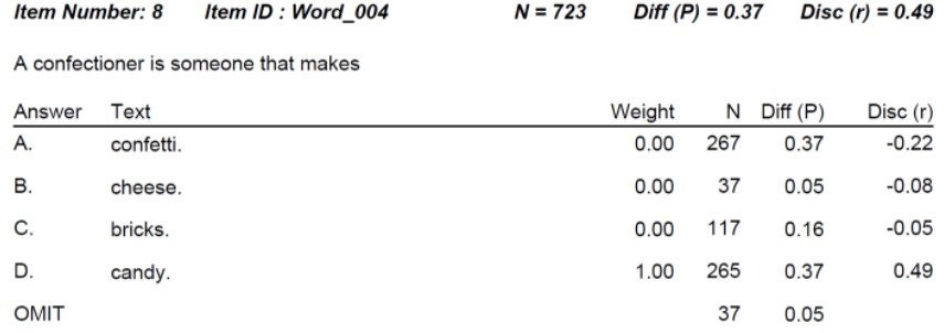
A simple example of item analysis is shown below.  This is an English vocabulary question.  This question is extremely difficult; only 37% of students get it correct even though there is a 25% chance just by guessing.  The item would probably be flagged for review.  However, the point-biserial discrimination is extremely high, telling us that the item is actually very strong and defensible.  Lots of students choose “confetti” but it is overwhelmingly the lower students, which is exactly what we want to have happen!

Confectioner-confetti

Where does a psychometrician work?

They work any place that develops high-quality tests.  Some examples:

  • Large educational assessment organizations like ACT
  • Governmental organizations like Singapore Examinations and Assessment Board
  • Professional certification and licensure boards like the International Federation of Boards of Biosafety
  • Employment testing companies like Biddle Consulting Group
  • Medical research like PROMIS
  • Universities like the University of Minnesota – mostly in purely academic roles
  • Language assessment groups like Berlitz
  • Testing services companies like ASC; such companies provide psychometric services and software to organizations that cannot afford to hire their own fulltime psychometrician.  This is often the case with certification and licensure boards.


What skills do I need?

There are two types of psychometrician: client-facing and data-facing.  Though many psychometricians have skills in both domains.

Client-facing psychometricians excel in what one of my former employers called Client Engagements; parts of the process where you work directly with subject matter experts and stakeholders.  Examples of this are job analysis studies, test design workshops, item writing workshops, and standard setting.  All of these involve the use of an expert panel to discuss certain aspects.  The skills you need here are soft skills; how to keep the SMEs engaged, meeting facilitation and management, explaining psychometric concepts to a lay person, and – yes – small talk during breaks!

Data-facing psychometricians focus on the numbers.  Examples of this include equating, item response theory analysis, classical test theory reports, and adaptive testing algorithms.  My previous employer called this the Client Reporting Team.  The skills you need here are quite different, and center around data analysis and writing code.


How do I get a job as a psychometrician?

First, you need a graduate degree.  In this field, a Master’s degree is considered entry-level, and a PhD is considered a standard level of education.  It can often be in a related area like I/O psychology.  Given that level of education, and the requirement for advanced data science skills, this career is extremely well-paid.

Wondering what kind of opportunities are out there?  Check out the NCME Job Board and Horizon Search, a headhunter for assessment professionals.

Are all they created equal?

Absolutely not!  Like any other profession, there are levels of expertise and skill.  I liken it to top-level athletes: there are huge differences between what constitutes a good football/basketball/whatever player in high school, college, and the professional level.  And the top levels are quite elite; many people who study psychometrics will never achieve them.

Personally, I group psychometricians into three levels:

Level 1: Practitioners at this level are perfectly comfortable with basic concepts and the use of classical test theory, evaluating items and distractors with P and Rpbis.  They also do client-facing work like Angoff studies; many Level 2 and Level 3 psychometricians do not enjoy this work.

Level 2: Practitioners at this level are familiar with advanced topics like item response theory, differential item functioning, and adaptive testing.  They routinely perform complex analyses with software such as Xcalibre.

Level 3: Practitioners at this level contribute to the field of psychometrics.  They invent new statistics/algorithms, develop new software, publish books, start successful companies, or otherwise impact the testing industry and science of psychometrics in some way.

Note that practitioners can certainly be extreme experts in other areas: someone can be an internationally recognized expert in Certification Accreditation or Pre-Employment Selection but only be a Level 1 psychometrician because that’s all that’s relevant for them.  They are a Level 3 in their home field.

Do these levels matter?  To some extent, they are just my musings.  But if you are hiring a psychometrician, either as a consultant or an employee, this differentiation is worth considering!
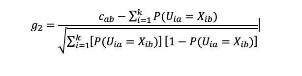
Confectioner-confetti

An item distractor, also known as a foil or a trap, is an incorrect option for a selected-response item on an assessment.

What makes a good item distractor?

One word: plausibility.  We need the item distractor to attract examinees.  If it is so irrelevant that no one considers it, then it does not do any good to include it in the item.  Consider the following item.


   What is the capital of the United States of America?

   A. Los Angeles

   B. New York

   C. Washington, D.C.

   D. Mexico City


The last option is quite implausible – not only is it outside the USA, but it mentions another country in the name, so no student is likely to select this.  This then becomes a three-horse race, and students have a 1 in 3 chance of guessing.  This certainly makes the item easier.

How much do distractors matter?  Well, how much is the difficulty affected by this new set?

   What is the capital of the United States of America?

   A. Paris

   B. Rome

   C. Washington, D.C.

   D. Mexico City


In addition, the distractor needs to have negative discrimination.  That is, while we want the correct answer to attract the more capable examinees, we want the distractors to attract the lower examinees.  If you have a distractor that you thought was incorrect, and it turns out to attract all the top students, you need to take a long, hard look at that question! To calculate discrimination statistics on distractors, you will need software such as Iteman.

What makes a bad item distractor?

Obviously, implausibility and negative discrimination are frequent offenders.  But if you think more deeply about plausibility, the key is actually plausibility without being arguably correct.  This can be a fine line to walk, and is a common source of problems for items.  You might have a medical item that presents a scenario and asks for a likely diagnosis; perhaps one of the distractors is very unlikely so as to be essentially implausible, but it might actually be possible for a small subset of patients under certain conditions.  If the author and item reviewers did not catch this, the examinees probably will, and this will be evident in the statistics.  This is one of the reasons it is important to do psychometric analysis of test results; in fact, accreditation standards often require you to go through this process at least once a year.