Psychometrics

Post-Training Assessment
Post-training assessment is an integral part of improving the performance and productivity of employees. To gauge the effectiveness of the training, assessments are the go-to solution for many businesses. They ensure transfer and retention of
Item Analysis in Psychometrics: Improve Your Test
Item analysis is the statistical evaluation of test questions to ensure they are good quality, and fix them if they are not. This is a key step in the test development cycle; after items have

Seven Technology Hacks to Deliver Assessments More Securely
So, yeah, the use of “hacks” in the title is definitely on the ironic and gratuitous side, but there is still a point to be made: are you making full use of current technology to
The IACAT Journal: JCAT
Do you conduct adaptive testing research? Perhaps a thesis or dissertation? Or maybe you have developed adaptive tests and have a technical report or validity study? I encourage you to check out the Journal of Computerized

Seguridad en exámenes y pruebas en línea
La seguridad y validez de las pruebas y exámenes en línea son extremadamente importantes. La pandemia COVID-19 cambió drásticamente todos los aspectos de nuestro mundo, y una de las áreas más afectadas es la evaluación

¿Qué es la vigilancia (proctoring) en línea?
La vigilancia en línea existe desde hace más de una década. Pero dado el reciente brote de COVID-19, las instituciones educativas y de fuerza laboral / certificación están luchando por cambiar sus operaciones, y una
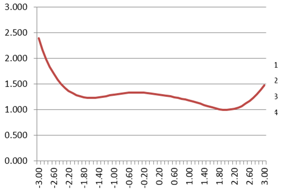
IRT Test Information Function
The IRT Test Information Function is a concept from item response theory (IRT) that is designed to evaluate how well an assessment differentiates examinees, and at what ranges of ability. For example, we might expect
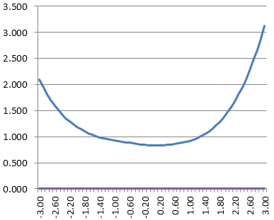
What Is The Standard Error of Measurement?
The standard error of measurement (SEM) is one of the core concepts in psychometrics. One of the primary assumptions of any assessment is that it is accurately and consistently measuring whatever it is we want

Question Banks: An Introduction
What is a question bank? A question bank refers to a pool of test questions to be used on various assessments across time. ..

Psychometrist: What do they do?
A psychometrist is a professional that specializes in how to deliver and interpret clinical psychological and educational assessments. That is, they work in a one-on-one clinical situation. For example, they might give IQ tests to

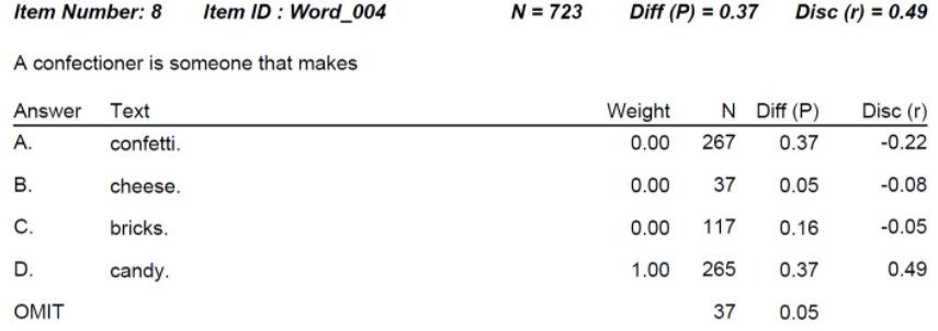
What is Classical Item Difficulty (P Value)?
One of the core concepts in psychometrics is item difficulty. This refers to the probability that examinees will get the item correct for educational/cognitive assessments or respond in the keyed direction with psychological/survey assessments (more on that

Item Banks: 6 Ways To Improve
The foundation of a decent assessment program is the ability to develop and manage strong item banks. Item banks are a central repository of test questions, each stored with important metadata such as Author or

Responses in Common (RIC) Index
This collusion detection (test cheating) index simply calculates the number of responses in common between a given pair of examinees. For example, both answered ‘B’ to a certain item regardless of whether it was correct

Exact Errors in Common (EEIC) collusion detection
Exact Errors in Common (EEIC) is an extremely basic collusion detection index simply calculates the number of responses in common between a given pair of examinees. For example, suppose two examinees got 80/100 correct on

Errors in Common (EIC) Exam Cheating Index
This exam cheating index (collusion detection) simply calculates the number of errors in common between a given pair of examinees. For example, two examinees got 80/100 correct, meaning 20 errors, and they answered all of
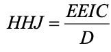
Harpp, Hogan, & Jennings (1996): Response Similarity Index
Harpp, Hogan, and Jennings (1996) revised their Response Similarity Index somewhat from Harpp and Hogan (1993). This produced a new equation for a statistic to detect collusion and other forms of exam cheating:. Explanation of
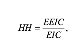
Harpp & Hogan (1993): Response Similarity Index
Harpp and Hogan (1993) suggested a response similarity index defined as Response Similarity Index Explanation EEIC denote the number of exact errors in common or identically wrong, EIC is the number of errors in common. This

Bellezza & Bellezza (1989): Error Similarity Analysis
This index evaluates error similarity analysis (ESA), namely estimating the probability that a given pair of examinees would have the same exact errors in common (EEIC), given the total number of errors they have in