Item Analysis and Statistics
Item analysis is the statistical evaluation of test questions to ensure they are good quality, and fix them if they are not. This is a key step in the test development cycle; after items have been delivered to examinees (either as a pilot, or in full usage), we analyze the statistics to determine if there are issues which affect validity and reliability, such as being too difficult or biased. This post will describe the basics of this process. If you’d like further detail and instructions on using software, you can also you can also check out our tutorial videos on our YouTube channel and download our free psychometric software.
Download a free copy of Iteman: Software for Item Analysis
What is Item Analysis?
Item analysis refers to the process of statistically analyzing assessment data to evaluate the quality and performance of your test items. This is an important step in the test development cycle, not only because it helps improve the quality of your test, but because it provides documentation for validity: evidence that your test performs well and score interpretations mean what you intend. It is one of the most common applications of psychometrics, by using item statistics to flag, diagnose, and fix the poorly performing items on a test. Every item that is poorly performing is potentially hurting the examinees.
Item analysis boils down to two goals:
- Find the items that are not performing well (difficulty and discrimination, usually)
- Figure out WHY those items are not performing well, so we can determine whether to revise or retire them
There are different ways to evaluate performance, such as whether the item is too difficult/easy, too confusing (not discriminating), miskeyed, or perhaps even biased to a minority group.
Moreover, there are two completely different paradigms for this analysis: classical test theory (CTT) and item response theory (IRT). On top of that, the analyses can differ based on whether the item is dichotomous (right/wrong) or polytomous (2 or more points).
Because of the possible variations, item analysis complex topic. But, that doesn’t even get into the evaluation of test performance. In this post, we’ll cover some of the basics for each theory, at the item level.
How to do Item Analysis
1. Prepare your data for item analysis
Most psychometric software utilizes a person x item matrix. That is, a data file where examinees are rows and items are columns. Sometimes, it is a sparse matrix where is a lot of missing data, like linear on the fly testing. You will also need to provide metadata to the software, such as your Item IDs, correct answers, item types, etc. The format for this will differ by software.
2. Run data through item analysis software
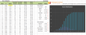
To implement item analysis, you should utilize dedicated software designed for this purpose. If you utilize an online assessment platform, it will provide you output for item analysis, such as distractor P values and point-biserials (if not, it isn’t a real assessment platform). In some cases, you might utilize standalone software. CITAS provides a simple spreadsheet-based approach to help you learn the basics, completely for free. A screenshot of the CITAS output is here. However, professionals will need a level above this. Iteman and Xcalibre are two specially-designed software programs from ASC for this purpose, one for CTT and one for IRT.
3. Interpret results of item analysis
Item analysis software will produce tables of numbers. Sometimes, these will be ugly ASCII-style tables from the 1980s. Sometimes, they will be beautiful Word docs with graphs and explanations. Either way, you need to interpret the statistics to determine which items have problems and how to fix them. The rest of this article will delve into that.
Item Analysis with Classical Test Theory
Classical Test Theory provides a simple and intuitive approach to item analysis. It utilizes nothing more complicated than proportions, averages, counts, and correlations. For this reason, it is useful for small-scale exams or use with groups that do not have psychometric expertise.
Item Difficulty: Dichotomous
CTT quantifies item difficulty for dichotomous items as the proportion (P value) of examinees that correctly answer it.
It ranges from 0.0 to 1.0. A high value means that the item is easy, and a low value means that the item is difficult. There are no hard and fast rules because interpretation can vary widely for different situations. For example, a test given at the beginning of the school year would be expected to have low statistics since the students have not yet been taught the material. On the other hand, a professional certification exam, where someone can not even sit unless they have 3 years of experience and a relevant degree, might have all items appear easy even though they are quite advanced topics! Here are some general guidelines”
0.95-1.0 = Too easy (not doing much good to differentiate examinees, which is really the purpose of assessment)
0.60-0.95 = Typical
0.40-0.60 = Hard
<0.40 = Too hard (consider that a 4 option multiple choice has a 25% chance of pure guessing)
With Iteman, you can set bounds to automatically flag items. The minimum P value bound represents what you consider the cut point for an item being too difficult. For a relatively easy test, you might specify 0.50 as a minimum, which means that 50% of the examinees have answered the item correctly.
For a test where we expect examinees to perform poorly, the minimum might be lowered to 0.4 or even 0.3. The minimum should take into account the possibility of guessing; if the item is multiple-choice with four options, there is a 25% chance of randomly guessing the answer, so the minimum should probably not be 0.20. The maximum P value represents the cut point for what you consider to be an item that is too easy. The primary consideration here is that if an item is so easy that nearly everyone gets it correct, it is not providing much information about the examinees. In fact, items with a P of 0.95 or higher typically have very poor point-biserial correlations.
Note that because the scale is inverted (lower value means higher difficulty), this is sometimes referred to as item facility.
The Item Mean (Polytomous)
This refers to an item that is scored with 2 or more point levels, like an essay scored on a 0-4 point rubric or a Likert-type item that is “Rate on a scale of 1 to 5.”
- 1=Strongly Disagree
- 2=Disagree
- 3=Neutral
- 4=Agree
- 5=Strongly Agree
The item mean is the average of the item responses converted to numeric values across all examinees. The range of the item mean is dependent on the number of categories and whether the item responses begin at 0. The interpretation of the item mean depends on the type of item (rating scale or partial credit). A good rating scale item will have an item mean close to ½ of the maximum, as this means that on average, examinees are not endorsing categories near the extremes of the continuum.
You will have to adjust for your own situation, but here is an example for the 5-point Likert-style item.
1-2 is very low; people disagree fairly strongly on average
2-3 is low to neutral; people tend to disagree on average
3-4 is neutral to high; people tend to agree on average
4-5 is very high; people agree fairly strongly on average
Iteman also provides flagging bounds for this statistic. The minimum item mean bound represents what you consider the cut point for the item mean being too low. The maximum item mean bound represents what you consider the cut point for the item mean being too high.
The number of categories for the items must be considered when setting the bounds of the minimum/maximum values. This is important as all items of a certain type (e.g., 3-category) might be flagged.
Item Discrimination: Dichotomous
In psychometrics, discrimination is a GOOD THING, even though the word often has a negative connotation in general. The entire point of an exam is to discriminate amongst examinees; smart students should get a high score and not-so-smart students should get a low score. If everyone gets the same score, there is no discrimination and no point in the exam! Item discrimination evaluates this concept.
CTT uses the point-biserial item-total correlation (Rpbis) as its primary statistic for this.
The Pearson point-biserial correlation (r-pbis) is a measure of the discrimination or differentiating strength, of the item. It ranges from −1.0 to 1.0 and is a correlation of item scores and total raw scores. If you consider a scored data matrix (multiple-choice items converted to 0/1 data), this would be the correlation between the item column and a column that is the sum of all item columns for each row (a person’s score).
A good item is able to differentiate between examinees of high and low ability yet have a higher point-biserial, but rarely above 0.50. A negative point-biserial is indicative of a very poor item because it means that the high-ability examinees are answering incorrectly, while the low examinees are answering it correctly, which of course would be bizarre, and therefore typically indicates that the specified correct answer is actually wrong. A point-biserial of 0.0 provides no differentiation between low-scoring and high-scoring examinees, essentially random “noise.” Here are some general guidelines on interpretation. Note that these assume a decent sample size; if you only have a small number of examinees, many item statistics will be flagged!
0.20+ = Good item; smarter examinees tend to get the item correct
0.10-0.20 = OK item; but probably review it
0.0-0.10 = Marginal item quality; should probably be revised or replaced
<0.0 = Terrible item; replace it
***Major red flag is if the correct answer has a negative Rpbis and a distractor has a positive Rpbis
The minimum item-total correlation bound represents the lowest discrimination you are willing to accept. This is typically a small positive number, like 0.10 or 0.20. If your sample size is small, it could possibly be reduced. The maximum item-total correlation bound is almost always 1.0, because it is typically desired that the Rpbis be as high as possible.
The biserial correlation is also a measure of the discrimination or differentiating strength, of the item. It ranges from −1.0 to 1.0. The biserial correlation is computed between the item and total score as if the item was a continuous measure of the trait. Since the biserial is an estimate of Pearson’s r it will be larger in absolute magnitude than the corresponding point-biserial.
The biserial makes the stricter assumption that the score distribution is normal. The biserial correlation is not recommended for traits where the score distribution is known to be non-normal (e.g., pathology).
Item Discrimination: Polytomous
The Pearson’s r correlation is the product-moment correlation between the item responses (as numeric values) and total score. It ranges from −1.0 to 1.0. The r correlation indexes the linear relationship between item score and total score and assumes that the item responses for an item form a continuous variable. The r correlation and the Rpbis are equivalent for a 2-category item, so guidelines for interpretation remain unchanged.
The minimum item-total correlation bound represents the lowest discrimination you are willing to accept. Since the typical r correlation (0.5) will be larger than the typical Rpbis (0.3) correlation, you may wish to set the lower bound higher for a test with polytomous items (0.2 to 0.3). If your sample size is small, it could possibly be reduced. The maximum item-total correlation bound is almost always 1.0, because it is typically desired that the Rpbis be as high as possible.
The eta coefficient is an additional index of discrimination computed using an analysis of variance with the item response as the independent variable and total score as the dependent variable. The eta coefficient is the ratio of the between-groups sum of squares to the total sum of squares and has a range of 0 to 1. The eta coefficient does not assume that the item responses are continuous and also does not assume a linear relationship between the item response and total score.
As a result, the eta coefficient will always be equal or greater than Pearson’s r. Note that the biserial correlation will be reported if the item has only 2 categories.
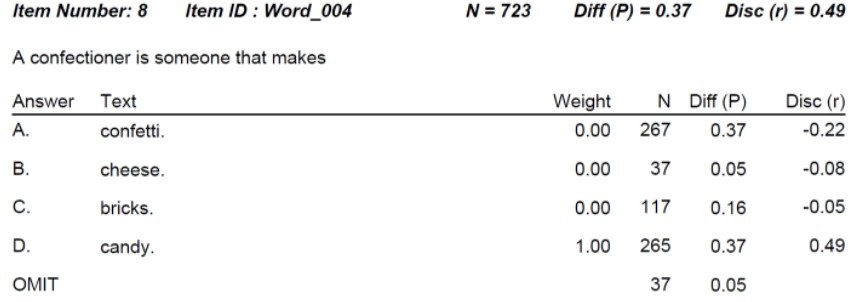
Key and Distractor Analysis
In the case of many item types, it pays to evaluate the answers. A distractor is an incorrect option. We want to make sure that more examinees are not selecting a distractor than the key (P value) and also that no distractor has higher discrimination. The latter would mean that smart students are selecting the wrong answer, and not-so-smart students are selecting what is supposedly correct. In some cases, the item is just bad. In others, the answer is just incorrectly recorded, perhaps by a typo. We call this a miskey of the item. In both cases, we want to flag the item and then dig into the distractor statistics to figure out what is wrong.
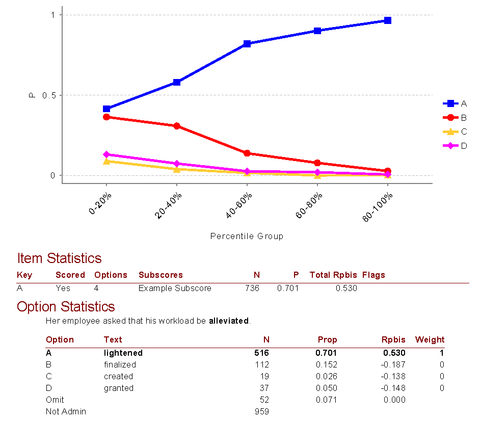
Example
Here is an example output for one item from our Iteman software, which you can download for free. You might also be interested in this video. This is a very well-performing item. Here are some key takeaways.
- This is a 4-option multiple choice item
- It was on a subscore named “Example subscore”
- This item was seen by 736 examinees
- 70% of students answered it correctly, so it was fairly easy, but not too easy
- The Rpbis was 0.53 which is extremely high; the item is good quality
- The line for the correct answer in the quantile plot has a clear positive slope, which reflects the high discrimination quality
- The proportion of examinees selecting the wrong answers was nicely distributed, not too high, and with negative Rpbis values. This means the distractors are sufficiently incorrect and not confusing.
Item Analysis with Item Response Theory
Item Response Theory (IRT) is a very sophisticated paradigm of item analysis and tackles numerous psychometric tasks, from item analysis to equating to adaptive testing. It requires much larger sample sizes than CTT (100-1000 responses per item) and extensive expertise (typically a PhD psychometrician). Maximum Likelihood Estimation (MLE) is a key concept in IRT used to estimate model parameters for better accuracy in assessments.
IRT isn’t suitable for small-scale exams like classroom quizzes. However, it is used by virtually every “real” exam you will take in your life, from K-12 benchmark exams to university admissions to professional certifications.
If you haven’t used IRT, I recommend you check out this blog post first.
Item Difficulty
IRT evaluates item difficulty for dichotomous items as a b-parameter, which is sort of like a z-score for the item on the bell curve: 0.0 is average, 2.0 is hard, and -2.0 is easy. (This can differ somewhat with the Rasch approach, which rescales everything.) In the case of polytomous items, there is a b-parameter for each threshold, or step between points.
Item Discrimination
IRT evaluates item discrimination by the slope of its item response function, which is called the a-parameter. Often, values above 0.80 are good and below 0.80 are less effective.
Key and Distractor Analysis
In the case of polytomous items, the multiple b-parameters provide an evaluation of the different answers. For dichotomous items, the IRT modeling does not distinguish amongst correct answers. Therefore, we utilize the CTT approach for distractor analysis. This remains extremely important for diagnosing issues in multiple choice items.
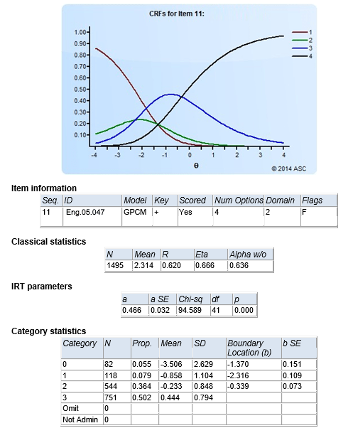
Example
Here is an example of what output from an IRT analysis program (Xcalibre) looks like. You might also be interested in this video.
- Here, we have a polytomous item, such as an essay scored from 0 to 3 points.
- It is calibrated with the generalized partial credit model.
- It has strong classical discrimination (0.62)
- It has poor IRT discrimination (0.466)
- The average raw score was 2.314 out of 3.0, so fairly easy
- There was a sufficient distribution of responses over the four point levels
- The boundary parameters are not in sequence; this item should be reviewed
Summary
This article is a very broad overview and does not do justice to the complexity of psychometrics and the art of diagnosing/revising items! I recommend that you download some of the item analysis software and start exploring your own data.
For additional reading, I recommend some of the common textbooks. For more on how to write/revise items, check out Haladyna (2004) and subsequent works. For item response theory, I highly recommend Embretson & Riese (2000).
Nathan Thompson, PhD
Latest posts by Nathan Thompson, PhD (see all)
- Situational Judgment Tests: Higher Fidelity in Pre-Employment Testing - November 30, 2024
- What is an Assessment-Based Certificate? - October 12, 2024
- What is Psychometrics? How does it improve assessment? - October 12, 2024