Psychometrics
What is Psychometrics? Definition, Examples, Careers
Psychometrics is the science of educational and psychological assessment, using data to ensure that tests are fair and accurate. Ever felt like you took a test which was unfair, too hard, didn’t cover the right

What is a Learning Management System (LMS)?
In today’s digital-first world, educational institutions and organizations are leveraging technology to deliver training and instruction in more dynamic and efficient ways. A core component of this shift is the Learning Management System (LMS). According

What is RIASEC Assessment? A tool to know yourself.
RIASEC assessment is type of personality assessment used to help individuals identify their career interests and strengths. Based on theory from John Holland, a renowned psychologist, this type of assessment is based on the premise
Factor Analysis: Evaluating Dimensionality in Assessment
Factor analysis is a statistical technique widely used in research to understand and evaluate the underlying structure of assessment data. In fields such as education, psychology, and medicine, this approach to unsupervised machine learning helps
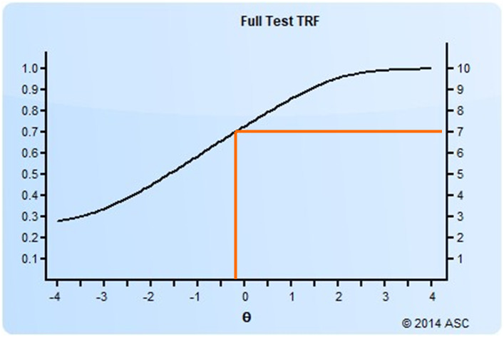
Setting a Cutscore to Item Response Theory
Setting a cutscore on a test scored with item response theory (IRT) requires some psychometric knowledge. This post will get you started. How do I set a cutscore with item response theory? There are two
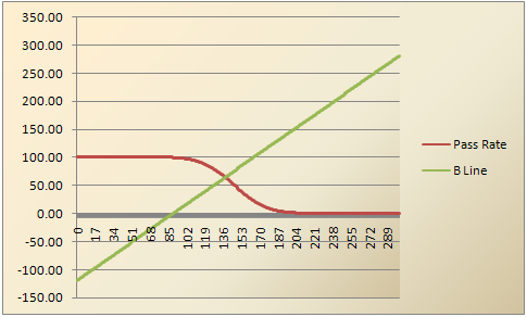
Modified-Angoff Method Study
A modified-Angoff method study is one of the most common ways to set a defensible cutscore on an exam. It therefore means that the pass/fail decisions made by the test are more trustworthy than if
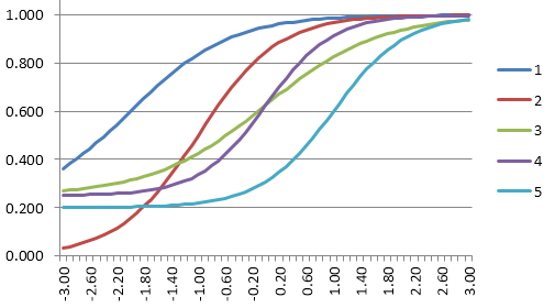
What is Item Response Theory (IRT)?
Item response theory (IRT) is a family of machine learning models in the field of psychometrics, which are used to design, analyze, validate, and score assessments. It is a very powerful psychometric paradigm that revolutionized

Criterion-related validity
Criterion-related validity is evidence that test scores are related to other data which we expect them to be. This is an essential part of the larger issue of test score validity, which is providing evidence

What is Digital Assessment, aka e-Assessment?
Digital assessment (DA) aka e-Assessment or electronic assessment is the delivery of assessments, tests, surveys, and other measures via digital devices such as computers, tablets, and mobile phones. The primary goal is to be able

Navigating Leadership Assessments: A Science-Backed Approach
Leadership assessments are psychometric tests used for selection, training, and promotion at work. They are more than just tools; they are crucial to identifying and developing effective organizational leadership. Plenty of options exist for “leadership

Why PARCC EBSR Items Provide Bad Data
The Partnership for Assessment of Readiness for College and Careers (PARCC) is a consortium of US States working together to develop educational assessments aligned with the Common Core State Standards. This is a daunting task,

What is Test Scaling?
Scaling is a psychometric term regarding the establishment of a score metric for a test, and it often has two meanings. First, it involves defining the method to operationally scoring the test, establishing an underlying

How do I develop a good Certification Test that meets standards?
Certification test development refers to the process of building an exam in accordance to international standards like NCCA, then delivering it securely. It is a critical business need for credentialing organizations and awarding bodies. As
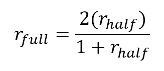
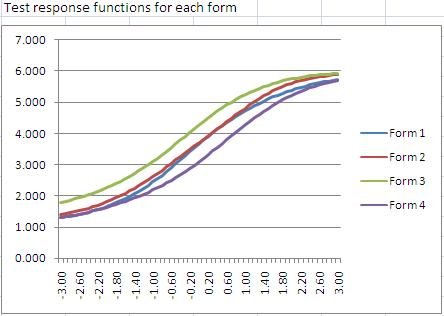
What is the Spearman-Brown formula?
The Spearman-Brown formula, also known as the Spearman-Brown Prophecy Formula or Correction, is a method used in evaluating test reliability. It is based on the idea that split-half reliability has better assumptions than coefficient alpha

Item Writing: Tips for Authoring Test Questions
Item writing (aka item authoring) is a science as well as an art, and if you have done it, you know just how challenging it can be! You are experts at what you do, and

Validity Threats and Psychometric Forensics
Validity threats are issues with a test or assessment that hinder the interpretations and use of scores, such as cheating, inappropriate use of scores, unfair preparation, or non-standardized delivery. It is important to establish a

Likert Scale Items
Likert scales (items) are a type of item used in human psychoeducational assessment, primarily to assess noncognitive constructs. That is, while item types like multiple choice or short answer are used to measure knowledge or

What are Test Blueprints & Specifications for Assessment?
Test blueprints, aka test specifications (shortened to “test specs”), are the formalized design of an assessment, test, or exam. This can be in the context of educational assessment, pre-employment, certification, licensure, or any other type.