What is Item Response Theory (IRT)?

Item response theory (IRT) is a family of machine learning models in the field of psychometrics, which are used to design, analyze, validate, and score assessments.  It is a very powerful psychometric paradigm that allows researchers to build stronger assessments, whether they work in Education, Psychology, Human Resources, or other fields.  It also solves critical measurement problems like equating across years, designing adaptive tests, or creating vertical scales.

Want to learn more about IRT, how it works, and why it is so important for assessment?  Read on.

What is Item Response Theory?

IRT is a family of models that try to describe how examinees respond to items on a test, hence the name.  These models can be used to evaluate item performance, because the descriptions are quite useful in and of themselves.  However, item response theory ended up doing so much more.

IRT is model-driven, in that there is a specific mathematical equation that is assumed, and we fit the models based on raw data, similar to linear regression.  There are different parameters (a, b, c) that shape this equation to different needs.  That’s what defines different IRT models.  This will be discussed at length below.

The models put people and items onto a latent scale, which is usually called θ (theta).  This represents whatever is being measured, whether IQ, anxiety, or knowledge of accounting laws in Croatia.  IRT helps us understand the nature of the scale, how a person answers each question, the distribution of item difficulty, and much more.  IRT used to be known as latent trait theory and item characteristic curve theory.

IRT requires specially-designed software.  Click the link below to download our software Xcalibre, which provides a user-friendly and visual platform for implementing IRT.

Why do we need Item Response Theory?

IRT represents an important innovation in the field of psychometrics. While now more than 50 years old – assuming the “birth” is the classic Lord and Novick (1969) text – it is still underutilized and remains a mystery to many practitioners.

Item response theory is more than just a way of analyzing exam data, it is a paradigm to drive the entire lifecycle of designing, building, delivering, scoring, and analyzing assessments.

• IRT helps us determine if a test is providing accurate scores on people, much more so than classical test theory.
• IRT helps us provide better feedback to examinees, which has far-reaching benefits for education and workforce development.
• IRT reduces bias in the instrument, through advanced techniques like differential item functioning.
• IRT maintains meaningful scores across time, known as equating.
• IRT can connect multiple levels of content, such as Math curriculum from Grades 3 to 12 if that is what you want to measure, known as vertical scaling within the progress monitoring framework.
• IRT is necessary to implement adaptive testing.
• IRT is particularly adept at handling a variety of test formats, including both speeded tests and power tests.

IRT requires larger sample sizes and is much more complex than its predecessor, classical test theory, but is also far more powerful.  IRT requires quite a lot of expertise, typically a PhD.  So it is not used for small assessments like a final exam at universities, but is used for almost all major assessments in the world.

The Driver: Problems with Classical Test Theory

Classical test theory (CTT) is approximately 100 years old, and still remains commonly used because it is appropriate for certain situations, and it is simple enough that it can be used by many people without formal training in psychometrics.  Most statistics are limited to means, proportions, and correlations.  However, its simplicity means that it lacks the sophistication to deal with a number of very important measurement problems.  A list of these is presented later.

Learn more about the differences between CTT and IRT here.

Item Response Theory Parameters

The foundation of IRT is a mathematical model defined by item parameters.  A parameter is an aspect of a mathematical model that can change its shape or other aspects.  For dichotomous items (those scored correct/incorrect), each item has three parameters:

   a: the discrimination parameter, an index of how well the item differentiates low from top examinees; typically ranges from 0 to 2, where higher is better, though not many items are above 1.0.

   b: the difficulty parameter, an index of what level of examinees for which the item is appropriate; typically ranges from -3 to +3, with 0 being an average examinee level.

   c: the pseudo-guessing parameter, which is a lower asymptote; typically is focused on 1/k where k is the number of options.

These paramters are used in the formula below, but are also displayed graphically.

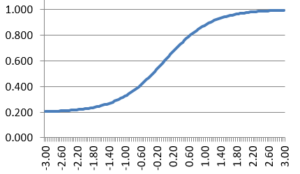
These parameters are used to graphically display an item response function (IRF), which models the probability of a correct answer as a function of ability.  In the example IRF, the a parameter is approximately, 1.0, indicating a fairly discriminating test item.  The b parameter is approximately 0.0 (the point on the x-axis where the midpoint of the curve is), indicating an average-difficulty item; examinees of average ability would have a 60% chance of answering correctly.  The c parameter is approximately 0.20, like a 5-option multiple choice item.  Consider the x-axis to be z-scores on a standard normal scale.

In some cases, there is no guessing involved, and we only use a and b.  This is called the two-parameter model.  If we only use b, this is the one-parameter or Rasch Model.  Here is how that is calculated.

Item parameters, which are crucial within the IRT framework, might change over time or multiple testing occasions, a phenomenon known as item parameter drift.

Example Item Response Theory calculations

Examinees with higher ability are much more likely to respond correctly.  Look at the graph above.  Someone at +2.0 (97th percentile) has about a 94% chance of getting the item correct.  Meanwhile, someone at -2.0 has only a 25% chance – barely above the 1 in 5 guessing rate of 20%.  An average person (0.0) has a 60% chance.  Why 60?  Because we are accounting for guessing.  If the curve went from 0% to 100% probability, then yes, the middle would be 50% change.  But here, we assume 20% as a baseline due to guessing, so halfway up is 60%.

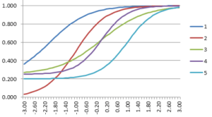
Of course, the parameters can and should differ from item to item, reflecting differences in item performance.  The following graph shows five IRFs with the three-parameter model.  The dark blue line is the easiest item, with a b of -2.00.  The light blue item is the hardest, with a b of +1.80.  The purple one has a c=0.00 while the light blue has c=0.25, indicating that it is more susceptible to guessing.

These IRFs are not just a pretty graph or a way to describe how an item performs.  They are the basic building block to accomplishing those important goals mentioned earlier.  That comes next…

Applications of Item Response Theory to Improve Assessment

Item response theory uses the IRF for several purposes.  Here are a few.

1. Interpreting and improving item performance
2. Scoring examinees with maximum likelihood or Bayesian methods
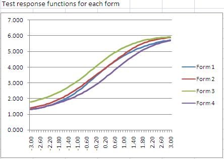
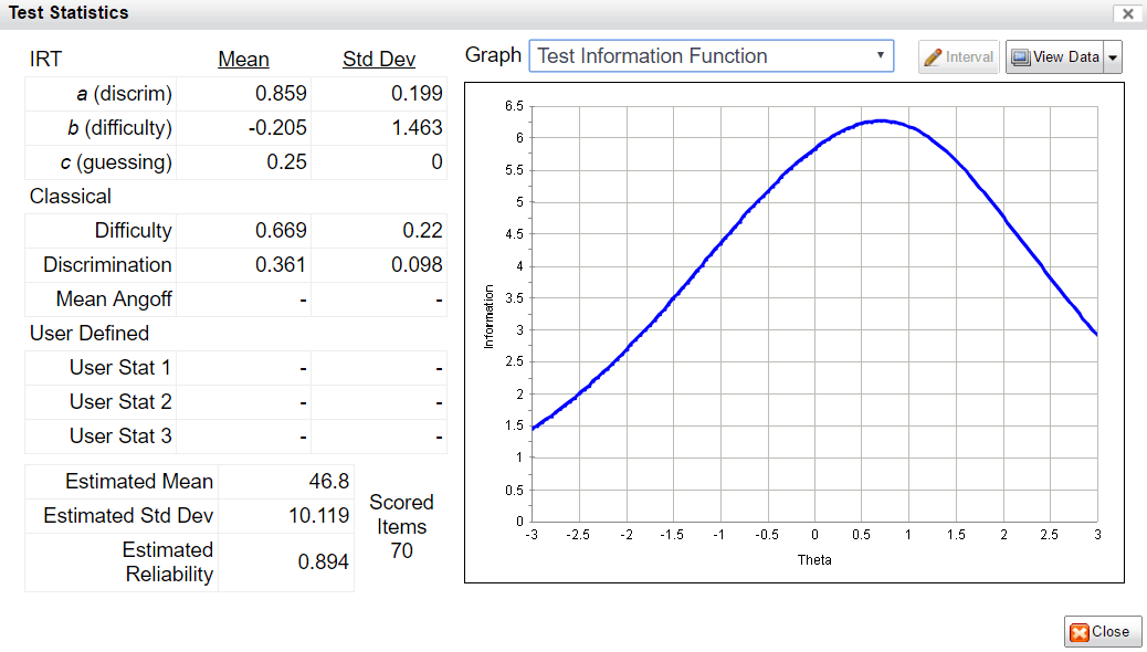
3. Form assembly, including linear on the fly testing (LOFT) and pre-equating
4. Calculating the accuracy of examinee scores
5. Development of computerized adaptive tests (CAT)
6. Post-equating
7. Differential item functioning (finding bias)
8. Data forensics to find cheaters or other issues

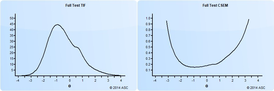
In addition to being used to evaluate each item individually, IRFs are combined in various ways to evaluate the overall test or form.  The two most important approaches are the conditional standard error of measurement (CSEM) and the test information function (TIF).  The test information function is higher where the test is providing more measurement information about examinees; if relatively low in a certain range of examinee ability, those examinees are not being measured accurately.  The CSEM is the inverse of the TIF, and has the interpretable advantage of being usable for confidence intervals; a person’s score plus or minus 1.96 times the SEM is a 95% confidence interval for their score.  The graph on the right shows part of the form assembly process in our  FastTest  platform.

Assumptions of Item Response Theory

Item response theory assumes a few things about your data.

1. The latent trait you are measuring is unidimensional.  If it is multidimensional, there is multidimensional item response theory, or you can treat the dimensions as separate traits.
2. Items have local independence, which means that the act of answering one is not impacted by others.  This affects the use of testlets and enemy items.
3. The probability of responding correctly to an item (or in a certain response, in the case of polytomous like Likert), is a function of the examinee’s ability/trait level and the parameters of the model, following the calculation of the item response function, with some allowance for random error.  As a corollary, we are assuming that the ability/trait has some distribution, with some people having higher or lower levels (e.g., intelligence) and that we are trying to find those differences.

Many texts will only postulate the first two as assumptions, because the third is just implicitly assumed.

Advantages and Benefits of Item Response Theory

So why does this matter?  Let’s go back to the problems with classical test theory.  Why is IRT better?

• Sample-independence of scale: Classical statistics are all sample dependent, and unusable on a different sample; results from IRT are sample-independent. within a linear transformation.  Two samples of different ability levels can be easily converted onto the same scale.
• Test statistics: Classical statistics are tied to a specific test form.
• Sparse matrices are OK: Classical test statistics do not work with sparse matrices introduced by multiple forms, linear on the fly testing, or adaptive testing.
• Linking/equating: Item response theory has much stronger equating, so if your exam has multiple forms, or if you deliver twice per year with a new form, you can have much greater validity in the comparability of scores.
• Measuring the range of students: Classical tests are built for the average student, and do not measure high or low students very well; conversely, statistics for very difficult or easy items are suspect.
• Vertical scaling: IRT can do vertical scaling but CTT cannot.
• Accounting for guessing: CTT does not account for guessing on multiple choice exams.
• Scoring: Scoring in classical test theory does not take into account item difficulty.  With IRT, you can score a student on any set of items and be sure it is on the same latent scale.
• Adaptive testing: CTT does not support adaptive testing in most cases.  Adaptive testing has its own list of benefits.
• Characterization of error: CTT assumes that every examinee has the same amount of error in their score (SEM); IRT recognizes that if the test is all middle-difficulty items, then low or high students will have inaccurate scores.
• Stronger form building: IRT has functionality to build forms to be more strongly equivalent and meet the purposes of the exam.
• Nonlinear function: IRT does not assume linear function of the student-item relationship when it is impossible.  CTT assumes a linear function (point-biserial) when it is blatantly impossible.

Item Response Theory Models: One Big Happy Family

Remember: IRT is actually a family of models, making flexible use of the parameters.  In some cases, only two (a,b) or one parameters (b) are used, depending on the type of assessment and fit of the data.  If there are multipoint items, such as Likert rating scales or partial credit items, the models are extended to include additional parameters. Learn more about the partial credit situation here.

Here’s a quick breakdown of the family tree, with the most common models.

• Unidimensional
  • Dichotomous
    • Rasch model
    • 1PL
    • 2PL
    • 3PL
    • 4PL (intellectual curiosity only!)
  • Polytomous
    • Rasch partial credit
    • Rasch rating scale
    • Generalized partial credit
    • Generalized rating scale
    • Graded response
• Multidimensional
  • Compensatory
  • Non-compensatory
  • Bifactor

How do I analyze my test with Item Response Theory?

First: you need to get special software.  There are some commercial packages like  Xcalibre, or you can use packages inside platforms like R and Python.

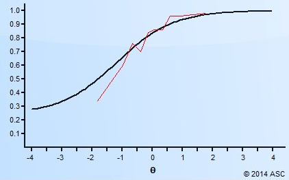
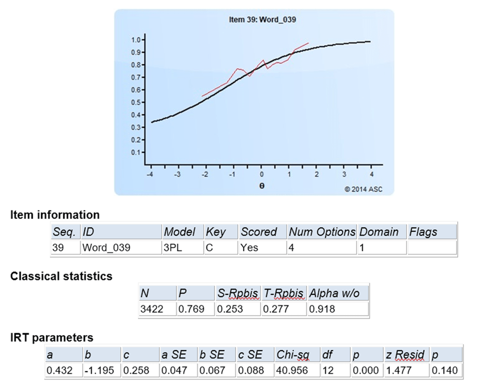
The software will analyze the data in cycles or loops to try to find the best model.  This is because, as always, the data does not always perfectly align.  You might see graphs like the one below if you compared actual proportions (red) to the predicted ones from the item response function (black).  That’s OK!  IRT is quite robust.  And there are analyses built in to help you evaluate model fit.

Some more unpacking of the image above:

• This was item #39 on the test
• We are using the three parameter logistic model (3PL), as this was a multiple choice item with 4 options
• 3422 examinees answered the item
• 76.9 of them got it correct
• The classical item discrimination (point biserial item-total correlation) was 0.253, which is OK but not very high
• The a parameter was 0.432, which is OK but not very strong
• The b parameter was -1.195, which means the item was quite easy
• The c parameter was 0.248, which you would expect if there was a 25% chance of guessing
• The Chi-square fit statistic rejected the null, indicating poor fit, but this statistic is susceptible to sample size
• The z-Resid fit statistic is a bit more robust, and it did not flag the item for bad fit

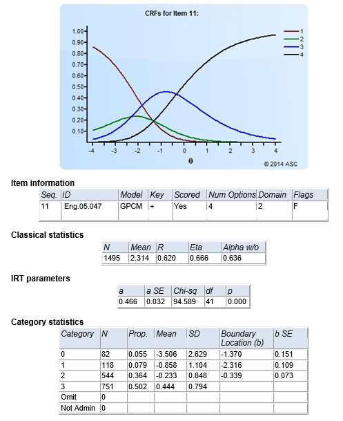
The image here shows output from  Xcalibre  from the generalized partial credit model, which is a polytomous model often used for items scored with partial credit.  For example, if a question lists 6 animals and asks students to click on the ones that are reptiles, of which there are 3.  The possible scores are then 0, 1, 2, 3.

Here, the graph labels them as 1-2-3-4, but the meaning is the same.  Here is how you can interpret this.

• Someone is likely to get 0 points if their theta is below -2.0 (bottom 3% or so of students).
• A few low students might get 1 point (green)
• Low-middle ability students are likely to get 2 correct (blue)
• Anyone above average (0.0) is likely to get all 3 correct.

The boundary locations are where one level becomes more likely than another, i.e., where the curves cross.  For example, you can see that the blue and black lines cross at the boundary -0.339.

Where can I learn more?

For more information, we recommend the textbook Item Response Theory for Psychologists by Embretson & Riese (2000) for those interested in a less mathematical treatment, or de Ayala (2009) for a more mathematical treatment.  If you really want to dive in, you can try the 3-volume Handbook of Item Response Theory edited by van der Linden, which contains a chapter discussing ASC’s IRT analysis software,  Xcalibre.

Want to talk to one of our experts about how to apply IRT?  Get in touch!

The following two tabs change content below.

• Bio
• Latest Posts

Nathan Thompson, PhD

Nathan Thompson earned his PhD in Psychometrics from the University of Minnesota, with a focus on computerized adaptive testing. His undergraduate degree was from Luther College with a triple major of Mathematics, Psychology, and Latin. He is primarily interested in the use of AI and software automation to augment and replace the work done by psychometricians, which has provided extensive experience in software design and programming. Dr. Thompson has published over 100 journal articles and conference presentations, but his favorite remains https://scholarworks.umass.edu/pare/vol16/iss1/1/ .

Latest posts by Nathan Thompson, PhD (see all)

• What is an Assessment-Based Certificate? - October 12, 2024
• What is Psychometrics? How does it improve assessment? - October 12, 2024
• What is RIASEC Assessment? - September 29, 2024