Psychometrics

Test Score Reliability and Validity
Test score reliability and validity are core concepts in the field of psychometrics and assessment. Both of them refer to the quality of a test, the scores it produces, and how we use those scores.

Progress Monitoring in Education
Progress monitoring is an essential component of a modern educational system and is often facilitated through Learning Management Systems (LMS), which streamline the tracking of learners’ academic achievements over time. Are you interested in tracking

What is Vertical Scaling in Assessment?
Vertical scaling in educational assessments is the process of placing scores that measure the same knowledge domain but at different ability levels onto a common scale (Tong & Kolen, 2008). The most common example is
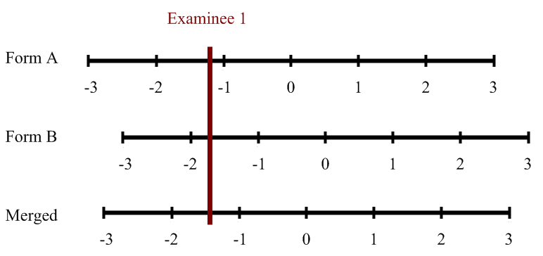
Test Score Equating and Linking
Test equating refers to the issue of defensibly translating scores from one test form to another. That is, if you have an exam where half of students see one set of items while the other

Examinee Collusion: Primary vs Secondary
In the field of psychometric forensics, examinee collusion refers to cases where an examinee takes a test with some sort of external help in obtaining the correct answers. There are several possibilities: The research on

What is the Positive Manifold?
Positive manifold refers to the fact that scores on cognitive assessment tend to correlate very highly with each other, indicating a common latent dimension that is very strong. This latent dimension became known as g for

The Bookmark Method of Standard Setting
The Bookmark Method of standard setting (Lewis, Mitzel, & Green, 1996) is a scientifically-based approach to setting cutscores on an examination. It allows stakeholders of an assessment to make decisions and classifications about examinees that

What is an Assessment / Test Battery?
A test battery or assessment battery is a set multiple psychometrically-distinct exams delivered in one administration. In some cases, these are various tests that are cobbled together for related purposes, such as a psychologist testing
Test Response Function in Item Response Theory
The Test Response Function (TRF) in item response theory (IRT) is a mathematical function that describes the relationship between the latent trait that a test is measuring, which psychometricians call theta (θ), and the predicted

What is a Psychometric Test or Assessment, and how do I select the right one?
Psychometric tests are assessments of people to measure psychological attributes such as personality or intelligence. They an increasingly important part in informing decisions about people in education, psychiatry, and employment/HR, as research shows they are

Three Approaches for IRT Equating
IRT equating is the process of equating test forms or item pools using item response theory to ensure that scores are comparable no matter what set of items that an examinee sees. If you are

The Rasch model
The Rasch model, also known as the one-parameter logistic model, was developed by Danish mathematician Georg Rasch and published in 1960. Over the ensuing years it has attracted many educational measurement specialists and psychometricians because

Paper-and-Pencil Testing: Still Around?
Paper-and-pencil testing used to be the only way to deliver assessments at scale. The introduction of computer-based testing (CBT) in the 1980s was a revelation – higher fidelity item types, immediate scoring & feedback, and

Power of linear on the fly testing
Linear on the fly testing (LOFT) is an approach to assessment delivery that increases test security by limiting item exposure. It tries to balance the advantages of linear testing (e.g., everyone sees the same number
Item-total point-biserial correlation
The item-total point-biserial correlation is a common psychometric index regarding the quality of a test item, namely how well it differentiates between examinees with high vs low ability. What is item discrimination? While the word
CalHR Selects Assessment Systems as Vendor for Personnel Selection
The California Department of Human Resources (CalHR, calhr.ca.gov/) has selected Assessment Systems Corporation (ASC, assess.com) as its vendor for an online assessment platform. CalHR is responsible for the personnel selection and hiring of many job roles for

What is a Standard Setting Study?
A standard setting study is a formal process for establishing a performance standard. In the assessment world, there are actually two uses of the word standard - the other one refers to...

What is Item Banking? What are Item Banks?
Item banking refers to the purposeful creation of a database of assessment items to serve as a central repository of all test content, improving efficiency and quality. The term item refers to what many call