Subject matter experts are an important part of the process in developing a defensible exam. There are several ways that their input is required. Here is a list from highest involvement/responsibility to lowest:
- Serving on the Certification Committee (if relevant) to decide important things like eligibility pathways
- Serving on panels for psychometric steps like Job Task Analysis or Standard Setting (Angoff)
- Writing and reviewing the test questions
- Answering the survey for the Job Task Analysis
Who are Subject Matter Experts?
A subject matter expert (SME) is someone with knowledge of the exam content. If you are developing a certification exam for widgetmakers, you need a panel of expert widgetmakers, and sometimes other stakeholders like widget factory managers.
You also need test development staff and psychometricians. Their job is to guide the process to meet international standards, and make the SME time the most efficient.
Example: Item Writing Workshop
 The most obvious usage of subject matter experts in exam development is item writing and review. Again, if you are making a certification exam for experienced widgetmakers, then only experienced widgetmakers know enough to write good items. In some cases, supervisors do as well, but then they are also SMEs. For example, I once worked on exams for ophthalmic technicians; some of the SMEs were ophthalmic technicians, but some of the SMEs (and much of the nonprofit board) were ophthalmologists, the medical doctors for whom the technicians worked.
An item writing workshop typically starts with training on item writing, including what makes a good item, terminology, and format. Item writers will then author questions, sometimes alone and sometimes as a group or in pairs. For higher stakes exams, all items will then be reviewed/edited by other SMEs.
Example: Job Task Analysis
Job Task Analysis studies are a key step in the development of a defensible certification program. It is the second step in the process, after the initial definition, and sets the stage for everything that comes afterward. Moreover, if you seek to get your certification accredited by organizations such as NCCA or ANSI, you need to re-perform the job task analysis study periodically. JTAs are sometimes called job analysis, practice analysis, or role delineation studies.
The job task analysis study relies heavily on the experience of Subject Matter Experts (SMEs), just like Cutscore studies. The SMEs have the best tabs on where the profession is evolving and what is most important, which is essential both for the initial JTA and the periodic re-set of the exam. The frequency depends on how quickly your field is evolving, but a cycle of 5 years is often recommended.
The goal of the job task analysis study is to gain quantitative data on the structure of the profession. Therefore, it typically utilizes a survey approach to gain data from as many professionals as possible. This starts with a group of SMEs generating an initial list of on-the-job tasks, categorizing them, and then publishing a survey. The end goal is a formal report with a blueprint of what knowledge, skills, and abilities (KSAs) are required for certification in a given role or field, and therefore what are the specifications of the certification test.
Observe— Typically the psychometrician (that’s us) shadows a representative sample of people who perform the job in question (chosen through Panel Composition) to observe and take notes. After the day(s) of observation, the SMEs sit down with the observer so that he or she may ask any clarifying questions.
The goal is to avoid doing this during the observation so that the observer has an untainted view of the job. Alternatively, your SMEs can observe job incumbents – which is often the case when the SMEs are supervisors.
- Generate— The SMEs now have a corpus of information on what is involved with the job, and generate a list of tasks that describe the most important job-related components. Not all job analysis uses tasks, but this is the most common approach in certification testing, hence you will often hear the term job task analysis as a general term.
Survey— Now that we have a list of tasks, we send a survey out to a larger group of SMEs and ask them to rate various features of each task.
How important is the task? How often is it performed? What larger category of tasks does it fall into?
Analyze— Next, we crunch the data and quantitatively evaluate the SMEs’ subjective ratings to determine which of the tasks and categories are most important.
Review— As a non-SME, the psychometrician needs to take their findings back to the SME panel to review the recommendation and make sure it makes sense.
Report— We put together a comprehensive report that outlines what the most important tasks/categories are for the given job. This in turn serves as the foundation for a test blueprint, because more important content deserves more weight on the test.
This connection is one of the fundamental links in the validity argument for an assessment.
Example: Cutscore studies
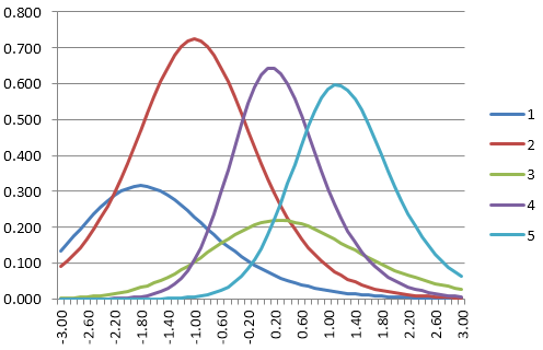
When the JTA is completed, we have to determine who should pass the assessment, and who should fail. This is most often done using the modified Angoff process, where the SMEs conceptualize a minimally competent candidate (MCC) and then set pass/fail point so that the MCC would just barely pass. There are other methods too, such as Bookmark or Contrasting Groups.
For newly-launching certification programs, these processes go hand-in-hand with item writing and review. The use of evidence-based practices in conducting the job task analysis, test design, writing items, and setting a cutscore serve as the basis for a good certification program. Moreover, if you are seeking to achieve accreditation – a third part stamp of approval that your credential is high quality – documentation that you completed all these steps is required.
Performing these tasks with a trained psychometrician inherently checks a lot of boxes on the accreditation to-do list, which can position your organization well for the future. When it comes to accreditation— the psychometricians and measurement specialists at Assessment Systems have been around the block a time or two. We can walk you through the lengthy process of becoming accredited, or we can help you perform these tasks a la carte.

 t all teachers had to use the “Chicago Method.” It was pure bunk and based on the fact that students should be doing as much busy work as possible instead of the teachers actually teaching. I think it is because some salesman convinced the department head to make the switch so that they would buy a thousand brand new textbooks. The method makes some decent points (